What interesting option could I explore to create the tiers within the
3 clusters (e.g. RFM quantile separation, classification algorithms)?
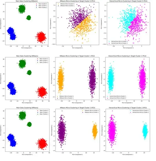
I'm late for this party but after generating synthetic data (with a bit challengeing nature not separted sample groups) with 3 main clusters as OP asked:
- cluster 0,
- cluster 1,
- and cluster 2
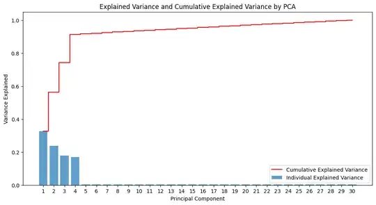
Then applying PCA to get the top 2 PCA: PCA Component 1 and PCA Component 2 with the main explained variance of info overall features.
 I have explored 2 proposed or potential solutions for micro clustering desired available main clusters
cluster_to_micro = 0  # Target one of the clusters
cluster_to_micro = 1
cluster_to_micro = 2
for proof of concept (PoC) and detail study of sued models performance for micro-clustering of potential sub-clusters. Please see the results:
import numpy as np
import pandas as pd
import matplotlib.pyplot as plt
from sklearn.datasets import make_blobs
from sklearn.decomposition import PCA
from sklearn.cluster import KMeans
from scipy.cluster.hierarchy import linkage, fcluster
Step 1: Generate synthetic data
n_customers = 5000
n_features = 30
#X, y_true = make_blobs(n_samples=n_customers, centers=5, n_features=n_features, random_state=42)
X, y_true = make_blobs(n_samples=n_customers,
                       centers=5,  # 5 centers for clearer substructure
                       n_features=n_features,
                       cluster_std=[2.0, 2.5, 1.5, 1.0, 1.8],  # Variable cluster spread
                       random_state=42)
df = pd.DataFrame(X, columns=[f"feature_{i}" for i in range(n_features)])
df['TrueCluster'] = y_true  # Assign true cluster labels for reference
Step 2: Apply PCA for dimensionality reduction
pca = PCA(n_components=2)  # Reduce to 2 components for visualization
X_pca = pca.fit_transform(X)
Step 3: Apply KMeans to identify initial clusters
kmeans = KMeans(n_clusters=3, random_state=42)  # 3 clusters at the top level
cluster_labels = kmeans.fit_predict(X_pca)
df['predicted_Cluster'] = cluster_labels  # Avoid data leakage by using a separate name
def visualize_micro_clustering(cluster_to_micro, X_pca, cluster_labels, df):
    # Focus on the target cluster (drop 'predicted_Cluster' for computations)
    target_cluster_data = df[df['predicted_Cluster'] == cluster_to_micro].drop(columns=['predicted_Cluster'])
# Apply PCA to target cluster
# Instead of dropping rows with NaNs, Impute NaNs with column means or 0 before applying PCA
# target_cluster_pca = PCA(n_components=2).fit_transform(target_cluster_data.iloc[:, :-1].dropna())  # Drop rows with NaNs
# Explicitly handle NaNs (replace with 0 in this example)
target_cluster_data_imputed = target_cluster_data.iloc[:, :-1].fillna(0)
target_cluster_pca = PCA(n_components=2).fit_transform(target_cluster_data_imputed)

# Apply KMeans for micro-clustering
kmeans_micro = KMeans(n_clusters=2, random_state=42)
df.loc[df['predicted_Cluster'] == cluster_to_micro, 'KMeansCluster'] = kmeans_micro.fit_predict(target_cluster_pca)

# Apply Hierarchical clustering for micro-clustering
linkage_matrix = linkage(target_cluster_pca, method='ward')
df.loc[df['predicted_Cluster'] == cluster_to_micro, 'HierarchicalCluster'] = fcluster(linkage_matrix, t=2, criterion='maxclust')

# Visualization
plt.figure(figsize=(18, 6))

# Main data clustering
plt.subplot(1, 3, 1)
main_colors = ['red', 'blue', 'green']
for main_cluster in range(3):
    main_subset = X_pca[cluster_labels == main_cluster]
    plt.scatter(main_subset[:, 0], main_subset[:, 1], alpha=0.6, label=f"Main Cluster {main_cluster}", color=main_colors[main_cluster])
plt.title(f"Main Data Clustering (KMeans)")
plt.xlabel("PCA Component 1")
plt.ylabel("PCA Component 2")
plt.legend()

# KMeans-based micro-clustering in target cluster
plt.subplot(1, 3, 2)
kmeans_colors = ['orange', 'purple']
for kmeans_cluster in [0, 1]:
    kmeans_subset = target_cluster_pca[df.loc[df['predicted_Cluster'] == cluster_to_micro, 'KMeansCluster'] == kmeans_cluster]
    plt.scatter(kmeans_subset[:, 0], kmeans_subset[:, 1], alpha=0.6, label=f"KMeans Micro-Cluster {kmeans_cluster}", color=kmeans_colors[kmeans_cluster])
plt.title(f"KMeans Micro-Clustering in Target Cluster {cluster_to_micro} (PCA)")
plt.xlabel("PCA Component 1")
plt.ylabel("PCA Component 2")
plt.legend()

# Hierarchical-based micro-clustering in target cluster
plt.subplot(1, 3, 3)
hierarchical_colors = ['cyan', 'magenta']
for hierarchical_cluster in [1, 2]:
    hierarchical_subset = target_cluster_pca[df.loc[df['predicted_Cluster'] == cluster_to_micro, 'HierarchicalCluster'] == hierarchical_cluster]
    plt.scatter(hierarchical_subset[:, 0], hierarchical_subset[:, 1], alpha=0.6, label=f"Hierarchical Micro-Cluster {hierarchical_cluster}", color=hierarchical_colors[hierarchical_cluster - 1])
plt.title(f"Hierarchical Micro-Clustering in Target Cluster {cluster_to_micro} (PCA)")
plt.xlabel("PCA Component 1")
plt.ylabel("PCA Component 2")
plt.legend()

plt.tight_layout()
plt.show()


Generate visualizations for all three clusters
for cluster_to_micro in [0, 1, 2]:
    visualize_micro_clustering(cluster_to_micro, X_pca, cluster_labels, df)
later you can apply from sklearn.metrics import silhouette_score, calinski_harabasz_score, davies_bouldin_score which performance was better to micro-cluster of potential sub-clusters witin main clusters better:
- sub-cluster 0
- sub-cluster 1
Hope this answer provides you possible options for your real data.

