HHL hermitian to unitary matrix convertation and output results

Question

I'm reading the paper describing the numerical example HHL. The first question related to the Hermitioan-unitary matrix transformation. We can use numpy.linalg.expm to convert Hermitian to unitary matrix - what I did and achieved the result that contradicts to one in paper:

$\begin{pmatrix} 0.51056242-0.79515385j & 0.27532484+0.17678405j \\ 0.27532484+0.17678405j & 0.51056242-0.79515385j \end{pmatrix}$

So, using this matrix, the further result also differs. What did I do wrong?

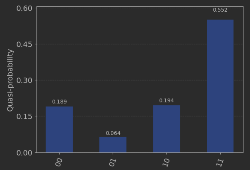
The second question is related to the result ration of the output vector $\vec{x}$. What the authors write about $\vec{x}$ is that

ratio of $|x_0|^2$ to $|x_1|^2$ is $1:9$.

however the output results show the different ratio: $0.142^2 : 0.361^2 = 1 : 2.54$

The question is resonable: what does the measured ration mean and how to make outcome to be more "true"?

The full code is below:

def qft_dagger(qc, n):
    for qubit in range(n//2): 
        qc.swap(qubit+1, n-qubit)
    for j in range(n):
        for m in range(j):
            qc.cp(np.pi/float(2**(j-m)), m+1, j+1)
        qc.h(j+1)
def qft(qc, n):
    for j in range(n):
        for m in range(j):
            qc.cp(-np.pi/float(2**(j-m)), clock[m], clock[j])
        qc.h(clock[n-j-1])
    for qubit in range(n//2):
        qc.swap(clock[qubit], clock[n-qubit-1])
def simulate(qpe):
    aer_sim = Aer.get_backend('aer_simulator')
    shots = 2048
    t_qpe = transpile(qpe, aer_sim)
    qobj = assemble(t_qpe, shots=shots)
    results = aer_sim.run(qobj).result()
    answer = results.get_counts()
    for k, v in answer.items():
      answer[k] = answer[k] / shots
    return answer
from qiskit.circuit import QuantumCircuit, QuantumRegister, ClassicalRegister, Parameter
from qiskit.circuit.library import UnitaryGate, CRYGate
from qiskit import Aer, transpile, assemble, execute
from qiskit.visualization import plot_histogram
import numpy as np
state = np.array([0, 1])
H = np.array([[1, -1/3], [-1/3, 1]])
U = np.array([[-1+1j, 1+1j], [1+1j, -1+1j]]) / 2
U_gate = UnitaryGate(U, 'U').control(1)
ancilla = QuantumRegister(1, 'ancilla')
clock = QuantumRegister(2, 'clock')
b = QuantumRegister(1, 'b')
classical = ClassicalRegister(2, 'classical')
circuit = QuantumCircuit(ancilla, clock, b, classical)
for q_idx in range(len(clock)):
    circuit.h(clock[q_idx])
circuit.prepare_state(state, b)
for q_idx in range(len(clock)):
    for _ in range(2**q_idx):
        circuit.append(U_gate, [q_idx + 1, b])
circuit.barrier()
qft(circuit, 2)
circuit.cry(np.pi, clock[0], ancilla)
circuit.cry(np.pi/3, clock[1], ancilla)
circuit.measure(ancilla, classical[0])
qft_dagger(circuit, 2)
circuit.barrier()
U = np.linalg.inv(U)
U_gate = UnitaryGate(U, 'U-1').control(1)
for q_idx in range(len(clock)):
    for _ in range(2**(len(clock) - q_idx - 1)):
        circuit.append(U_gate, [len(clock) - q_idx, b])
circuit.barrier()
for q_idx in range(len(clock)):
    circuit.h(clock[q_idx])
circuit.barrier()
circuit.measure(b, classical[1])
measurements = simulate(circuit)
plot_histogram(measurements)

the results are the same as in the paper:

diemilio · Accepted Answer · 2024-10-07T15:17:38.777

The difference between what you have and what is in the paper is that you are calculating the matrix $U = e^{iA}$, and in the paper they calculate: $ U = e^{iAt},$ with $t=3\pi/4$.

The reason they do this is because they already know what the solution is going to be, so they are basically rescaling the matrix $A$ to given them "nicer" eigenvalues that allow them to cheat in the implementation of the eigenvalue inversion step.

As for why your solution is not giving the 1:9 ratio, it could be that if you are using the same angles as used in the paper for the eigenvalue inversion step but your matrix is $U = e^{iA}$, then your result is obviously going to be incorrect because you haven't accounted for the $3\pi/4$ scaling for the angles.

HHL hermitian to unitary matrix convertation and output results

1 Answers1