Using a slightly different but equivalent notation, the radius of the distorted point as a function of the undistorted point is described by the following equation:
\begin{aligned}
f(r) = r + k_1 r^3 + k_2 r^5
\end{aligned}
where $r = \sqrt{x^2 + y^2}$.
Problem Statement
Given $x', y'$, let $r' = \sqrt{x'^2 + y'^2}$. Find $r \in f^{-1}(r')$, after which $x = \frac{r}{r'} \cdot x'$ and $y = \frac{r}{r'} \cdot y'$ (in the special case where $r' = 0$, $x = x'$ and $y = y'$).
General Solution
The solutions to the problem are all the real roots of the polynomial $f(r) - r' = k_2 r^5 + k_1 r^3 + r - r'$. There is no closed-form solution for the roots of a quintic function, but there are software solutions available in various programming languages that provide numerical estimates (Python, R, C++, MATLAB, Mathematica, etc.). Many of these solutions rely on the Jenkins-Traub algorithm.
Alternative (Simpler) Methods
When Is $f$ Invertible?
For many realistic values of $(k_1, k_2)$, it turns out that $f$ is an invertible function, which means we can find a unique solution for any $r'$. In some applications, ensuring that $f$ is invertible is important. The following observations allow us to understand when $f$ is invertible:
- $f'(0) = 1$, which means that $f$ is strictly increasing at $r = 0$.
- $f'$ has real roots if and only if $k_2 \leq g(k_1)$, where
\begin{aligned}
g(k_1) = \begin{cases}
\frac{9}{20}k_1^2 & ~\text{if}~k_1 < 0, \\
0 & ~\text{otherwise}.
\end{cases}
\end{aligned}
I'll omit the proof of the second bullet, but it can be derived by applying the quadratic formula to $f'(r)$ after the substitution $u = r^2$.
It follows from the second bullet that $f$ is strictly monotone (and therefore invertible) if and only if $k_2 \geq g(k_1)$. The first bullet further implies that if $f$ is invertible, then it is also strictly increasing.
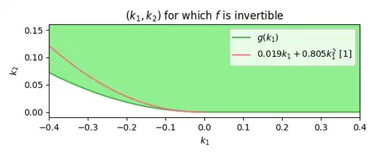
According to Figure 3 in [1], the majority of empirically measured lens distortion coefficients fall within the region for which $f$ is invertible. Below, I've plotted the empirical curve from the paper (red) along with the region of valid coefficients (green).
Method 1: Bisection Search (Guaranteed Convergence Under Loose Conditions)
If $f$ is invertible, we may use a simple bisection search to find $\hat{r} \approx f^{-1}(r')$ with error tolerance $\left|f(\hat{r}) - r'\right| \leq \tau$. The actual conditions for convergence using the bisection search algorithm presented in this section may be relaxed to the following:
Important: This algorithm is guaranteed to terminate only if either $\bf k_2 > 0$ or $\bf \left( k_1 \geq 0 ~and~ k_2 \geq 0 \right)$. For computational reasons, I recommend ensuring that $k_2 > \varepsilon$ for a small $\varepsilon > 0$ when $k_1 < 0$. These conditions assure us that $\lim_{r \uparrow \infty} f(r) = \infty$, which guarantees that an upper bound for the bisection search will be established (referring to $r_u$ in the algorithm below). Keep in mind that applying this to a non-invertible $f$, i.e., when $k_2 < g(k_1)$, means the solution is not guaranteed to be unique. Note that this algorithm may also be applied to higher-order polynomial radial distortion models and is guaranteed to converge as long as the highest-order coefficient is positive.
function $f^{-1}(r'; \tau)$:
$\phantom{{}++{}}r_l \gets 0$
$\phantom{{}++{}}r_u \gets 2 \cdot r'$
$\phantom{{}++{}}$while $f(r_u) < r'$
$\phantom{{}++++{}}r_l \gets r_u$
$\phantom{{}++++{}}r_u \gets 2 \cdot r_u$
$\phantom{{}++{}}\hat{r} \gets \frac{1}{2} \cdot (r_l + r_u)$
$\phantom{{}++{}}q \gets f(\hat{r})$
$\phantom{{}++{}}$while $\left| q - r' \right| > \tau$
$\phantom{{}++++{}}$if $q > r'$ then $r_u \gets \hat{r}$ else $r_l \gets \hat{r}$
$\phantom{{}++++{}}\hat{r} \gets \frac{1}{2} \cdot (r_l + r_u)$
$\phantom{{}++++{}}q \gets f(\hat{r})$
$\phantom{{}++{}}$return $\hat{r}$
Method 2: Simple Iterative Method (Without Convergence Guarantees)
Source: As far as I can tell, the algorithm presented in this section was originally presented here. It is also the method used by the OpenCV undistortPoints function (method not documented but can be verified by looking at the source code).
This method has the benefit of being extremely simple to implement and converges quickly for relatively small amounts of distortion. If applying a fixed number of iterations without convergence testing, this is also a differentiable operation, which may be necessary for certain applications.
We can intuitively understand the method from the observation that the original equation may be reorganized to
\begin{equation}
r = \frac{r'}{1 + k_1 r^2 + k_2 r^4}
\end{equation}
which gives rise to the iteration
\begin{equation}
r_{0} := r', ~~~r_{n+1} := \frac{r'}{1 + k_1 r_{n}^2 + k_2 r_{n}^4}.
\end{equation}
While this usually converges for small and moderate distortion, it won't always converge for large distortions, even when $f$ is invertible. For example, if $(k_1, k_2) = (-0.4, 0.12)$ and $r' = 2$, we get oscillatory behavior as seen in the following figure:

The method can be augmented to operate with a reduced step size. For example, let $\alpha \in (0, 1]$, then
\begin{equation}
r_{0} := r', ~~~r_{n+1} := (1 - \alpha) \cdot r_{n} + \alpha \cdot \frac{r'}{1 + k_1 r_{n}^2 + k_2 r_{n}^4}.
\end{equation}
Unfortunately, a good value for $\alpha$ depends on the specific values of $k_1$, $k_2$, and $r'$. I have yet to work out a bound on $\alpha$ or a schedule that guarantees convergence. Based on empirical testing, I propose the conjecture that there exists some $\alpha$ that will always result in convergence, though choosing $\alpha$ too small results in very slow convergence.
function $f^{-1}(r'; N, \alpha, \tau)$:
$\phantom{{}++{}}\hat{r} \gets r'$
$\phantom{{}++{}}n \gets 0$
$\phantom{{}++{}}$while $\left|f(\hat{r}) - r'\right| > \tau$ and $n < N$
$\phantom{{}++++{}}\hat{r} \gets (1 - \alpha) \cdot \hat{r} + \alpha \cdot r' / \left(1 + k_1\cdot \hat{r}^2 + k_2\cdot \hat{r}^4 \right)$
$\phantom{{}++++{}}n \gets n + 1$
$\phantom{{}++{}}$return $\hat{r}$
For reference, the parameters that result in behavior equivalent to OpenCV are $N = 10$, $\alpha = 1$, and $\tau = 0$.
[1] Lopez, M., Mari, R., Gargallo, P., Kuang, Y., Gonzalez-Jimenez, J., & Haro, G. (2019). Deep single image camera calibration with radial distortion. In Proceedings of the IEEE Conference on Computer Vision and Pattern Recognition (pp. 11817-11825).

