I was taught that the forward formula should be used when calculating the value of a point near $x_0$ and the backward one when calculating near $x_n$. However, the interpolation polynomial is unique, so the value should be the same. So is there any difference between the two, or my lecturer is wrong?
Here are the formulas:
- Gregory-Newton or Newton Forward Difference Interpolation $$P(x_{0}+hs)=f_{0}+s\Delta f_{0}+\frac{s(s-1)}{2!}\Delta^{2}f_{0}+\cdots+\frac{s(s-1)(s-2)...(s-n+1)}{n!}\Delta^{n}f_{0}$$ where $$s=\frac{(x-x_{0})}{h}; \qquad f_0=f(x_0); \qquad \Delta^k f_i=\sum_{j=0}^k{(-1)^j \frac{k!}{j!(k-j)!}f_{i+k-j}}$$
- Gregory-Newton or Newton Backward Difference Interpolation $$P(x_{n}+hs)=f_{n}+s\nabla f_{n}+\frac{s(s+1)}{2!}\nabla^{2}f_{n}+\cdots+\frac{s(s+1)(s+2)...(s+n-1)}{n!}\nabla^{n}f_{n}$$ where $$s=\frac{(x-x_{n})}{h}; \qquad f_n=f(x_n); \qquad \nabla^k f_i=\sum_{j=0}^k{(-1)^j \frac{k!}{j!(k-j)!}f_{i-j}}$$
Example: For interpolating at the points $x_0=-3,-2.9,-2.8,...,2.9,3=x_n$ with $f(x)=e^x$ using MATLAB we have
>> x = -3:0.1:3; y = exp(x);
>> frwrdiffdata = frwrdiff(x, y, 0.1, -3:0.5:3);
>> bckwrdiffdata = bkwrdiff(x, y, 0.1, -3:0.5:3);
>> mostAccurateData = exp(-3:0.5:3)';
>> [abs(frwrdiffdata-mostAccurateData)./mostAccurateData ...
abs(bckwrdiffdata-mostAccurateData)./mostAccurateData]

ans =

   1.0e-03 *

                   0   0.672871398134864
   0.000000000000169   0.001123487151044
   0.000000000000205   0.000000247108705
                   0   0.000000006452206
   0.000000000000302   0.000000000010412
   0.000000000000366   0.000000000005491
   0.000000000000222   0.000000000001776
   0.000000000000135                   0
   0.000000000000327   0.000000000000327
   0.000000000093342                   0
   0.000000006938894                   0
   0.000003364235903                   0
   0.000053772150047                   0
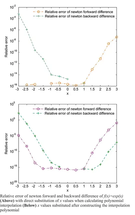
where the first column is the relative error of Newton Forward Difference and the second column is the relative error of Newton Backward Difference for sample points $x=-3,-2.5,-2,...,2.5,3$. As you see in the table above and in the following figure the relative error in the first column increases as $x\to x_n$ and the relative error of the second column decreases as $x\to x_n$.
The MATLAB functions frwrdiff and bkwrdiffused above are
function polyvals = frwrdiff(x, y, h, p) % Newton Forward Difference function
n = length(x);
ps = length(p);
polyvals = zeros(ps, 1);
dd = zeros(n,n);
dd(:, 1) = y(:);
for i = 2: n % divided diference table
    for j = 2: i
        dd(i,j) = (dd(i, j-1) - dd(i-1, j-1));
    end
end
a = diag(dd); %y_0, delta_0, ..., delta_n
for k = 1: ps
    s = (p(k) - x(1))/h; %(x - x_0) / h
    t = s;
    polyvals(k) = a(1) + s*a(2); %y_0 + s * delta_0
    for i = 1: n-2
       t = t * (s - i);
       polyvals(k) = polyvals(k) + t*a(i+2)/factorial(i+1);
    end
end
and
function polyvals = bkwrdiff(x, y, h, p) % Newton Backward Difference function
n = length(x);
ps = length(p);
polyvals = zeros(ps, 1);
dd = zeros(n,n);
dd(:, 1) = y(:);
for i = 2: n % divided diference table
    for j = 2: i
        dd(i,j) = (dd(i, j-1) - dd(i-1, j-1));
    end
end
a = dd(n,:); %y_n, nabla_0, ..., nabla_n
for k = 1: ps
    s = (p(k) - x(n))/h; %(x - x_n) / h
    t = s;
    polyvals(k) = a(1) + s*a(2); %y_0 + s * nabla_0
    for i = 1: n-2
       t = t * (s + i);
       polyvals(k) = polyvals(k) + t*a(i+2)/factorial(i+1);
    end
end
Note: The results seem different when at first we obtain the polynomials and then substitute the points $x=-3,-2.5,-2,...,2.5,3$ to the polynomials:
ans =

   1.0e+02 *

   0.000000132146955   1.528566476043447
   0.000000000047960   0.000683674054800
   0.000000000000000   0.000000095605754
   0.000000000000000   0.000000000002139
   0.000000000000000   0.000000000000000
   0.000000000000000   0.000000000000000
   0.000000000000000                   0
   0.000000000000000                   0
   0.000000000000000   0.000000000000000
   0.000000000000331   0.000000000000000
   0.000000004277456   0.000000000000000
   0.000006632407337   0.000000000000896
   0.001154767626752   0.000000000785245
The above results obtained by modifying the two matlab functions already mentioned in this question.