Runge-Kutta method accuracy

Question

I got a Runge-Kutta method here and I solve this system using it.

So here's Runge-Kutta stuff \begin{align} k_1 &= f(t_n, y_n) \\ k_2 &= f(t_n + h/2, y_n + hk_1/2) \\ k_3 &= f(t_n+h, y_n - hk_1 + 2hk_2) \\\hline y_{n+1} &= y_n + h(k_1 + 4k_2 + k_3)/6 \end{align} where $h$ is step

Here's my test system \begin{align} y'_1 &= -5y_1 - 10y_2 + 14e^{-x} \\ y'_2 &= -10y_1 - 5y_2 + 14e^{-x} \end{align} with exact solution $y_1(x) = y_2(x) = e^{-x}$

UPD: The initial condition here is $y_1(0) = y_2(0) = 1$

I need to solve it on $[0;4]$.

---

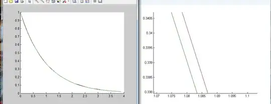
Well, I thought I solved it right, because I checked how the exact solution and these approximate solution plots looks like (on the left, on the right I zoomed plot until saw difference)

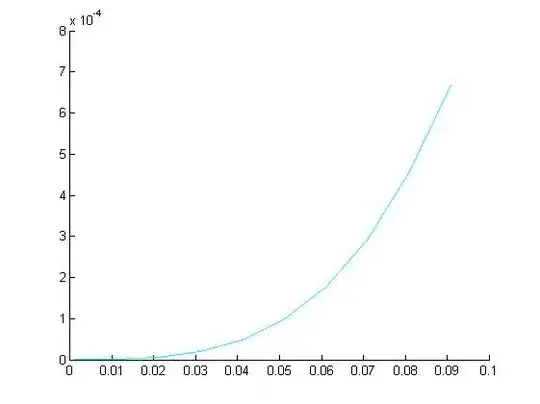
Also I checked how the plot of the difference between exact solution and approximate solution depending on step (let's call it e/h) looks like.

So $e/h$ it looks like this

But when I checked e/h^4 dependence it looked like these

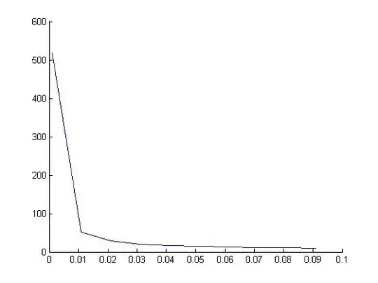
I showed it to the teacher and she said that my solution is wrong, it's not suppose to be like these! I show my code to her asked for help but she said that she doesn't understand matlab :c

Have I really done something wrong? And if yes what I've done wrong? And if not how to prove that I'm right?

Here's my code btw

Runge-Kutta method

  function [ res_y ] = RungeKutta(dim, size, grid, step, f1,f2,y1, y2)
k1=zeros(dim);
k2=zeros(dim);
k3=zeros(dim);

h = step;

res_y(1,1) = y1;
res_y(2,1) = y2;

for i=1: size

   k1(1)= f1(grid(i),y1,y2);
   k1(2)= f2(grid(i),y1,y2);

   k2(1)= f1(grid(i)+h/2, y1+h*k1(1)/2, y2+h*k1(2)/2);
   k2(2)= f2(grid(i)+h/2, y1+h*k1(1)/2, y2+h*k1(2)/2);

   k3(1)= f1(grid(i)+h, y1-h*k1(1)+2*h*k2(1), y2-h*k1(2)+2*h*k2(2));
   k3(2)= f2(grid(i)+h, y1-h*k1(1)+2*h*k2(1), y2-h*k1(2)+2*h*k2(2));

   res_y(1,i+1) = y1 + h*(k1(1) + 4*k2(1) + k3(1))/6;
   res_y(2,i+1) = y1 + h*(k1(2) + 4*k2(2) + k3(2))/6;

   y1 = res_y(1,i+1); 
   y2 = res_y(2,i+1);
end


end

Main method

    a = 0; b = 4;
    h = 0.1; % step
    t = a:h:b; %grid
    n = 2; 
    m = size(t,2);
 hold on;
     plot(t, exp(-t),'b-')
     plot(t, exp(-t),'r--')
 hold off;

y1=1; y2 = 1;

f1_ptr = @f1;% out = -5 * y1 - 10 * y2 + (14)*exp(-x);
f2_ptr = @f2;% out = -10 * y1 - 5 * y2 + (14)*exp(-x);

res_y = RungeKutta(n,m-1,t,h,f1_ptr, f2_ptr,1,1);

hold on;
plot(t,res_y);

hold off;


%e/h and e/h^4 plots
fig_a = figure;
set(fig_a,'name','e/h','numbertitle','off')
hold on;
counter = 0;
for h=0.001:0.01:0.1
    y1=1; y2 = 1;
    t = a:h:b;
    m = size(t,2);
    counter = counter + 1;
result_appr = RungeKutta(n,m-1,t,h,f1_ptr, f2_ptr,y1,y2);
result_exact = exp(-t);



result_difference = abs(result_appr(1, :) - result_exact);
e1(counter) = max(result_difference);
e2(counter) = max(result_difference);

hh = h*h*h*h;

ehh1(counter)=e1(counter)/hh;
ehh2(counter)=e2(counter)/hh;  



end;
h=0.001:0.01:0.1;
    plot(h,e1,'c');
    plot(h,e2,'c');
hold off;
fig_b = figure;
set(fig_b ,'name','e/h^4','numbertitle','off')
hold on;
    plot(h,ehh1,'r')
    plot(h,ehh2,'b')
hold off;

f1 function

function [ out ] = f1( x, y1, y2, alpha, beta )
if nargin == 3
    alpha = 5;
    beta = 10;
end
out = -alpha * y1 - beta * y2 + (alpha + beta - 1)*exp(-x);
end

f2 function

function [ out ] = f2( x, y1, y2, alpha, beta )
if nargin == 3
    alpha = 5;
    beta = 10;
end
out = -beta * y1 - alpha * y2 + (alpha + beta - 1)*exp(-x);
end

Answer 1

The method is a classical third-order method as computed and presented by M. Wilhelm Kutta in 1901, based on the Simpson quadrature rule.

This means that the global error will scale like $h^3$ and the local truncation error like $h^4$.

Plotting the error as computed against $h$, but in a loglog plot and for a geometric sequence of step sizes, for h = 10.^[-4:0.5:-1], gives a line that has a very nice slope $3$.

Another way to visualize this is to plot the difference of the computed to the exact solution divided by $h^3$. This gives an error profile plot

that nicely and visually converges to the leading coefficient $c(x)$ in $e(x)=c(x)h^3+O(h^4)$. Note that this is the absolute error, and that the solutions fall exponentially to zero, which explains that the error falls in the end. In a plot of the relative error one could expect the curve to continue to grow away from zero.