Let us consider a prototypal case (see figure)
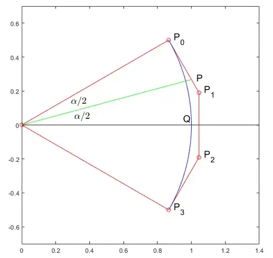
Fig. 1.
where we assume :
that there exist a line of symmetry making $P_2$ and $P_3$ the images of $P_1$ and $P_0$ resp.
that, moreover, up to a rotation, a translation and a homothety, point $P_0$ can be chosen WLOG with coordinates
$$(a,b)=(\cos \alpha,\sin \alpha) \ \ \text{ where} \ \ 0<\alpha<\pi/2.$$
In this way, the issue is reduced to understand how $P_1$ must be chosen knowing $\alpha$.
We are going to show that the ideal option is by choosing $P_1$ on the orthogonal line $(\ell)$ to $OP_0$ issued from $P_0$ such that $\vec{P_0P_1}=\tfrac43 \vec{P_0P}$ where $P$ is the point on line $(\ell)$ such that $\angle POP_0=\tfrac12 \alpha$.
Otherwise said :
$$\underbrace{\|\vec{P_0P_1}\|}_k=\tfrac43 \tan(\tfrac12 \alpha)\tag{1}$$
Here is why.
Let us write the expression of the cubic Bézier under the form :
$$M=s^3P_0+3s^2tP_1+3st^2\overline{P_1}+t^3\overline{P_0} \ \ \text{where} \ \ s:=1-t$$
Let us expand it :
$$M=s^3(a+ib)+3s^2t(a+ib-ki(a+ib))+3st^2(a-ib+ki(a-ib))+t^3(a-ib)\tag{2}$$
Now consider the case where $M$ is the midpoint $Q$ of the arc (case $s=t=\tfrac12$).
One can consider that the circularity will be optimal by constraining $Q$ to be at abscissa $\color{red}{1}$ on the $x$ axis. In this way we will have $OQ=OP_0=OP_3=1$.
Taking $s=t=\tfrac12$ in (2) gives :
$$\tfrac18((a+ib)+3(a+kb)+3(a+kb)+(a-ib))=\color{red}{1}$$
Setting $a=\cos \alpha, \ b=\sin \alpha$, we get
$$8 \cos \alpha + 6 k \sin \alpha = 8$$
$$k=\frac{4(1- \cos \alpha)}{3 \sin \alpha}$$
$$k=\frac{4 \times 2 \sin^2(\alpha/2)}{3 \times 2 \sin (\alpha/2) \cos(\alpha/2)}$$
Simplifying, one gets the value of $k$ given in (1).
It is interesting to have an idea of the local (and global) discrepancy of the Bezier arc wrt to a circular arc. it is represented on Fig. 2. In the case of angle $\alpha=\tfrac{\pi}{6}$ taken in Fig. 1, one sees that the relative maximal discrepancy is good ($\approx 2.5 \times 10^{-5}$).
Remark : I just had a look at this reference given by @PM 2Ring giving exactly the same expression (2), though with a different approach.
Even better approximations could be achieved, by moving very slightly $P_0, Q, P_3$ as explained in this reference. But my personal opinion is that it is not useful because it is so easy to have exact circular arcs by turning to rational Bézier curves !
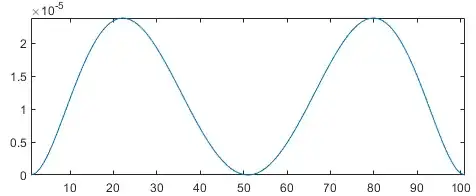
Fig. 2.
Appendix : Matlab program for the generation of Fig. 1 and Fig. 2 :
 clear all;close all;
 an=pi/6;k=(4/3)*tan(an/2);P0=exp(i*an);P3=conj(P0);
 P1=(1-k*i)*P0;P2=conj(P1);
 PP=[P0,P1,P2,P3];
 p=0.7;plot([0,2*p],[0,0],'-k');hold on;
 plot([0,PP,0],'-or');axis equal;axis([0,2*p,-p,p])
 t=0:0.01:1;s=1-t;
 f=PP*[s.^3;3*s.^2.*t;3*s.*t.^2;t.^3];plot(f,'b'); % cubic Bézier
 P=1+i*tan(an/2);
 plot([0,P],'-g');
 Q=0.92+0.03i;L=[PP,P,Q];
 set(gcf,'defaulttextfontsize',15)
 text(real(L)+0.03,imag(L)+0.01,{'P_0','P_1','P_2','P_3','P','Q'});
 text([0.29,0.31],[0.14,0.05],{'$\alpha/2$','$\alpha/2$'},'Interpreter','latex');
 figure
 plot(abs(f)-1)

