Rectifying radial lens distortion

Question

I have an image with lens distortion determined with 7 radial distortion terms $k_1$ thru $k_7$ calculated using the collinearity equation given by

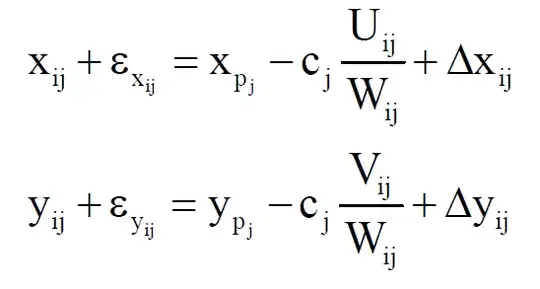
where the lens distortion is given by

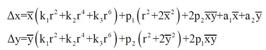
Since the tangential distortion terms are negligible, and ignoring scale $a_1$ and shear $a_2$ terms, I am only left with radial distortion.

I am having a difficult time trying to rectify the image from the lens distortion, and so far is have tried to estimate the $x$ and $y$ directly and using the radial distances method.

Based on the method suggested here, I considered the radial distance model where

$$r{'}= r+k_1r^{3}+k_2r^{5}+...+k_7r^{15}$$

where $r=\sqrt{(x-x_p)^2 + (y-y_p)^2}$ and tried to solve for $r$ using Newton method

where $f(r) = r+k_1r^{3}+k_2r^{5}+...+k_7r^{15} - r{'}$ and $f'(r) = 1+3k_1r{2}+5k_2r^{4}+...+15k_7r^{14}$ but the resultant image doesn't look ok. Python implementation :

def undistort_radial_newton_raphson (img, K, dist):
    rectified_img = np.ones_like(img)
    xp = K[0,2]
    yp = K[1,2]
    c = K[0,0]
    k1, k2, p1, p2, k3, k4, k5,k6, k7 = dist
for x in range(img.shape[1]):
    for y in range(img.shape[0]):
        xbar = x - xp
        ybar = y - yp
    rdash = np.sqrt(xbar**2 + ybar**2)

    r = rdash

    for _ in range(100):
        f_r = r + k1*r**3 + k2*r**5 + k3*r**7 + k4*r**9 + k5*r**11+ k6*r**13 + k7*r**15 - rdash

        f_d_r = 1 + 3*k1*r**2 + 5*k2*r**4 + 7*k3*r**6 +\
                    9*k4*r**8 + 11*k5*r**10 + 13*k6*r**12 + 15*k7*r**14

        r_new = r - (f_r/f_d_r)

        delta = np.abs(r_new - r)

        r = r_new

        if delta <= 1e-6:
            break

    xu = ((r/rdash) * x)
    yu = ((r/rdash) * y)

    if ((xu >= 0) and (xu < img.shape[1])) and (((yu >= 0) and (yu < img.shape[0]))):
       rectified_img[int(yu), int(xu), :] =  img[y, x, :]



fig, axes = plt.subplots(1, 2)
axes[0].imshow(img)
axes[0].set_title("Distorted image")
axes[0].axis('off')
axes[1].imshow(rectified_img)
axes[1].set_title("Rectified image")
axes[1].axis('off')
axes[1].grid(color='w')
Adjust layout and show plot
plt.tight_layout()
plt.show()

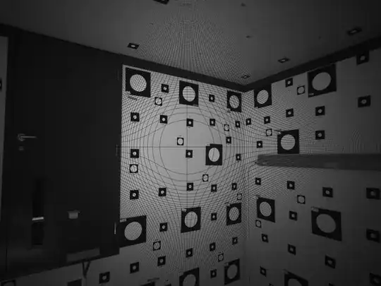
Result:

I am not sure what I am missing. Additionally I also tried

1. Applied the bisection algorithm mention in 1 but with only 1st 6 coefficients, that didn't work
2. Applied Newton's method using the collinearity eq and the result was
3. I just calculated $\Delta x$ and $\Delta y$ and subtracted it from $x'$ and $y'$ to result in

I'm really unable to figure out what I am missing or where I am going wrong. Anything really helps.

Thanks

Data to recreate:

calib_params ={
    'xp': 1003.031205,
    'yp': 789.486771,
    'c': 1161.8444,
    'k1': -3.338358E-07,
    'k2': 1.347146E-13,
    'k3': -1.521870E-18,
    'p1':   3.081290E-08,
    'p2':   9.872170E-08,
    'k4':   3.585315E-24,
    'k5':   -4.688132E-30,
    'k6':   3.019413E-36,
    'k7':   -7.996873E-43,
}