10

Consider the random experiment in which $y_{-1}, y_{+1}$ are i.i.d. exponential random variables with rate parameter $\lambda$, sampled at $x=-1$ and $x=1$, respectively. For each sample, consider the lines passing through the points $(-1, y_{-1})$ and $(-1, y_{+1})$, with opposite, fixed slopes (positive and negative, respectively). We then construct a piecewise-linear function $y(x)$ joining the point $(-1,y_{-1})$ to the intersection of the two lines, then to $(1,y_{+1})$, forming a "corner".

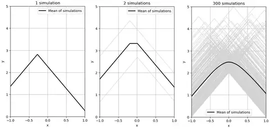
After repeating this experiment many times, the average of these piecewise-linear plots forms an empirical curve, as seen below

enter image description here

Is it possible to derive an explicit expression for this expected curve, $\mathbb{E}[y(x)]$, over the interval $-1 \le x \le 1$?

sam wolfe
  • 3,465

2 Answers2

6

We will assume here that the slope of the line emanating from $(-1,y_{-1})$ is $t>0$. First, note that in the interval $[-1,1]$, the graph produced by realizations of the random variables $y_{-1}:=a, y_1:=b$ with PDF $f(x), x\geq 0$ can be written piecewise

$$y_{a,b}(x)=\begin{Bmatrix}(t(x+1)+a)\theta(x-\frac{b-a}{2t})+(t(1-x)+b)\theta(-x+\frac{b-a}{2t})&|b-a|\leq 2t\\t(x+1)+a&b-a>2t\\ t(1-x)+b&b-a<-2t\end{Bmatrix}$$ where the Heaviside function has been used to reduce clutter. This problem now reduces to computing the integral

$$E[y(x)]=\int_{[0,\infty]^2}dadbf(a)f(b)y_{a,b}(x)=\int_{-\infty}^{+\infty}dD\int^\infty_{\max(0,-D)}f(A)f(D+A)y_{A, D+A}(x)dA$$

where in the second equality we performed the change of variables $D=b-a, A=a$, which simplifies the regions of $y(x)$ considerably. Due to the presence of the max function in the inner integral, we have to split the integrand according to the sign of $D$ as well. After considering all possible regions and massaging, one can show that

$$E[y(x)]_{x>0}=\int_{0}^{\infty}dD\int_{0}^{\infty}dAf(A)f(D+A)(t(1+x)+A)+ \\\int^{0}_{-\infty}dD\int_{-D}^{\infty}dAf(A)f(D+A)(t(1-x)+D+A)+\int_{0}^{2tx}dD\int_{0}^{\infty}dAf(A)f(D+A)(D-2tx)$$

$$E[y(x)]_{x<0}=\int_{0}^{\infty}dD\int_{0}^{\infty}dAf(A)f(D+A)(t(1+x)+A)+ \\\int^{0}_{-\infty}dD\int_{-D}^{\infty}dAf(A)f(D+A)(t(1-x)+D+A)+\int^{0}_{2tx}dD\int_{-D}^{\infty}dAf(A)f(D+A)(2tx-D)$$

For $a,b\sim \text{Exp}(\lambda)$, the integrals are elementary, yielding the tidy result

$$E[y(x)]=t+\frac{1}{2\lambda}+\frac{1-2\lambda t|x|-e^{-2\lambda t|x|}}{2\lambda}$$

It is not hard to show that the expectation value is $C^2(-1,1)$, so its graph appears smooth.
  • Thanks! Just one quick question, at $x=\pm 1$, shouldn't we get $E[y(\pm1)]=\frac{1}{\lambda}$, since $y(\pm1)=y_{\pm 1}\sim \text{Exp}(\lambda)$? – sam wolfe Mar 16 '25 at 00:21
  • 1
    Now that I think of it, perhaps not, since there might be cases where a line starting at $x=-1$, for example, reaches $x=1$ "before" $y_1$ is sampled resulting in a lower image at $x=1$. Is this correct? – sam wolfe Mar 16 '25 at 00:29
  • Not in this setup. I take into account lines that intersect outside of the interval $(-1,1)$. If you want to that condition to hold, you have to use sampling that rejects those- but from looking at your plot showing multiple simulations, it seems like you did not. – K. Grammatikos Mar 16 '25 at 00:29
  • 1
    Makes sense. We indeed get $\lim_{t\to\infty}E[y(\pm 1)]=\frac{1}{\lambda}$, and $\lim_{t\to\infty}E[y(x)]=\infty$ for $x\in (-1,1)$, as expected. Thank you so much! – sam wolfe Mar 16 '25 at 00:44
  • Interestingly, in a simplified case, these curves are related to the curve $|x|+e^{-|x|}$. I'm wondering how far this curve is from a catenary, or other interesting curves, within $(-1,1)$. Generally wondering if there is something more interesting about this curve. $C^2(-1,1)$ is a nice result, for example. Anyway, this is beyond the scope of this question, but I'll leave this comment here. – sam wolfe Mar 16 '25 at 01:19
0

For each value of $x$, it is possible to obtain an expression for $\mathbb E[y(x)]$ involving integrals with respect to the exponential density, but these integrals would I think have to be evaluated numerically.

Let the slopes of the lines be $\alpha$ and $-\alpha$. The piecewise linear function $f^i(x)$ for the $i$'th observation can be written as the minimum of the two straight lines:

$f^i(x) = \min \left([y^i_{-1} + \alpha (x+1)], [y^i_{+1} - \alpha (x-1)]\right)$

The minimum above is the second straight line if

$[y^i_{-1} + \alpha (x+1)] > [y^i_{+1} - \alpha (x-1)] \iff 2 \alpha x > y^i_{+1} - y^i_{-1}$

Let $A^i$ be the event $2 \alpha x > y^i_{+1} - y^i_{-1}$ and let $1_A^i$ denote the indicator function of this event. The functions $f^i(x)$ can be rewritten using $1_A^i$, and then the average function $f(x)=\mathbb E[y(x)]$ can be written as $\mathbb E[f^i(x)]$ to yield the following expression:

$$\mathbb E[y(x)] = \mathbb E(f^i(x)) = \mathbb E\left[(1-1_A^i) (y^i_{-1} + \alpha (x+1)) + 1_A^i (y^i_{+1} - \alpha (x-1))\right] = \mathbb E\left[y^i_{-1} + \alpha (x+1) - 1_A^i y^i_{-1} -1_A^i \alpha x - 1_A^i \alpha + 1_A^i y^i_{+1} - 1_A^i \alpha x - 1_A^i \alpha\right]$$

The above expression involves the following kinds of terms all of which require at most a univariate numerical integration:

  • Expectation of the exponential variable $y^i_{-1}$ which is available in closed form.
  • Known constants like $\alpha (x+1)$ and $\alpha x$
  • Expectation of $1_A^i y^i_{-1}$. For a fixed value of $y^i_{-1}$, the conditional probability that $1_A^i=1$ is given by the cumulative distribution function of an exponential variable. Multiplying this by the probability density function of $y^i_{-1}$ and integrating gives this expectation. This is a univariate integral which has to be computed numerically. The same analysis applies to $1_A^i y^i_{+1}$.
  • Expectation of $1_A^i$ (times a constant like $\alpha$).The density function of the difference of two exponential variables can be obtained in closed form similar to the standard formula for the sum of two independent exponential random variables. So these computations involve only a univariate integral with respect to this density.