Reflection between Two Parallel Cylinders

Question

I am interested in the following question.

Consider two identical cylinders (or in 2D, two circles) of radius $r$, with centers separated by a distance $s$. A point particle is released above with a vertical downward velocity, its initial horizontal offset measured by the distance $\xi $ from the midline between the cylinders. The particle travels in straight lines between reflections and undergoes perfectly elastic collisions (i.e. the angle of incidence equals the angle of reflection) with the cylinders’ surfaces.

In the figures below, the parameters are set to $ r = 140 $ and $ s = 300 $.

Clearly, when the particle is exactly in the middle ($ \xi = 0 $), it passes straight through.

When the particle is offset from the middle by a certain amount (e.g. $ \xi = 30 $), it is reflected back.

It appears that there is a critical case in between where the particle bounces infinitely many times between the two cylinders. On one side of this critical case, the particle eventually escapes downwards (as $ t \to \infty $, $ y \to \infty $); on the other side, the particle is reflected back (as $ t \to \infty $, $ y \to -\infty $). Below is the case $ \xi = 21.21$, slightly above the critical case.

Using the bisection method, the critical value $ \xi_c $ under these parameters is found to be approximately $21.20735102$.

My knowledge in dynamical systems is relatively limited. Through some research, I found that this is a type of billiard system. The phenomenon at the critical case appears to be related to chaotic dynamics. Nonetheless, the system gives me a sense of being very simple, intuitive, and, in a sense, "monotonic." This problem appears to possess a certain "locality"—that is, the most crucial aspect is the reflection behavior at the point where the two cylinders are closest. This gives me hope that there might be a way to derive a closed-form solution.

My question is: Can we obtain any closed-form solution for this critical value? If a closed-form solution seems unattainable, is there any other way to mathematically characterize this critical case?

Answer 1

Partial analysis of the asymptotic case.

Let’s parameterize the problem by assuming the circles are unit circles with a distance of $d$ between them at their closest (the centers are $d+2$ apart).

Also, let’s just consider the bounces between the middle and the right side.

Let $(y_n,m_n)$ be the absolute slope and height when the the ball passes through the middle on the $n$th time, assume that $y_n,m_n \ll 1$ and let’s ignore all 2nd order effects.

Then, the line will hit the circle at $x$ location (up to 2nd order) $d/2$ and height $z_n=y_n+m_n d/2$.

Then, the circle on the right has slope $1/z_n$, so the slope of the reflection will be (up to 2nd order) $-(m_n+2z_n)$. Thus, we find that:

$$z_n=y_n +m_n d/2$$ $$m_{n+1}=m_n+2z_n$$ $$y_{n+1}=y_n+(m_n+m_{n+1})d/2 $$

Simplifying gives:

$$m_{n+1}=(1+d)m_n +2 y_n$$ $$y_{n+1}=((1+d/2)d)m_n+(1+d)y_n$$

This linear recurrence has eigenvalues $1+d\pm \sqrt{2d+d^2}$. The two roots are inverses of each other. Then, adjacent jumps will get exponentially smaller towards flat and with less distance between each other with the ratio between adjacent jumps and slopes being those eigenvalues.

The eigenvectors are $(1,\pm \sqrt{2d+d^2}/2)$, so that’ll be the ratio between the slope and height. This has the nice consequence that lines near the middle, if extended, will go approximately through the points $(\pm \sqrt{2d+d^2}/2,0)$ which can be verified visibly in the OP’s diagrams.

If this fact were to hold for all ranges, then you’d get an easy answer of the vertical asymptote being directly above one of these points. Unfortunately, the nonlinearities of the problem break this invariant, so approximation is probably your best bet (although maybe there’s a different nice analytic invariant that makes the problem approachable).

Answer 2

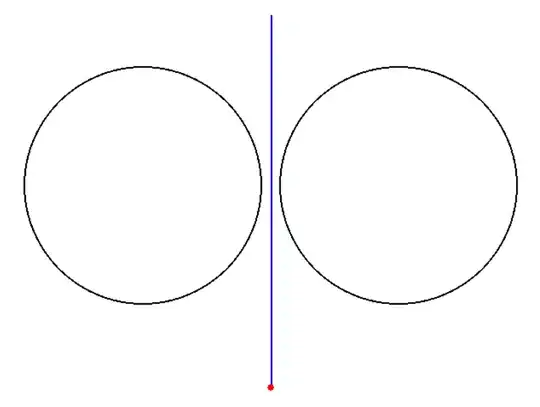
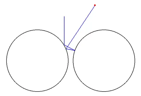
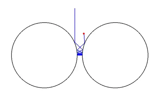
Here is a numerical calculation that can help characterize the critical position. Now, the problem is scale-invariant, so let us assume that the radius of the cylinders is 1, and let the distance between their centers be expressed as a multiple of the radius. (If we need to scale up this problem, we can simply multiply all of the distances involved by the new radius, which will not affect the qualitative bouncing behavior at all.)

Then the problem really only has one parameter, $d\geq 2$, the distance between the cylinder centers (expressed as a multiple of the radius). And given that distance $d$, we can compute the critical $x$-position from which to fire the initial ray so that earlier positions all escape upward and later positions all escape downward. That critical value is a function of $s$ alone.

Here is a numerically calculated plot, using binary search as before:

Note that I'm using a coordinate system centered on one of the cylinders, instead of centered on the midpoint between them. This is so that the critical point is always a number between 0 and 1 (ranging from the midpoint of the cylinder all the way to one side).

Of course I hope that my calculations are correct; one reality check is that the critical value approaches $1/\sqrt{2}$ from below as the distance between the cylinders grows large. And indeed, an initial ray fired downward at $x=\frac{1}{\sqrt{2}}$ will reflect off the $45^\circ$ normal in a horizontal line straight toward the other cylinder. This makes sense: as the distance becomes large relative to the radius, the first reflected ray must get closer and closer to horizontal to even have a chance of hitting the other cylinder at such a great distance, let alone re-reflecting at a helpful angle.

---

Finally, the qualitative behavior I observe:

1. The function has an asymptotically vertical slope line as you approach d=2 from the right. (Similar to the behavior of the sqrt function.)
2. The function's leftmost endpoint is (2,1)
3. The function has a horizontal asymptote of 1/sqrt(2) toward +infinity.
4. The function is monotonically decreasing everywhere.

I have puzzled over what functional form qualitatively captures this effect, and have not yet discovered a satisfying answer. A curve like $$f(x) \approx 1 + \left(\frac{1}{\sqrt{2}}-1\right)\sqrt{\frac{x-2}{x}}$$ has the correct qualitative endpoint behavior but is not the best fit for small values of $x$.

As a test case, when $r=140$ and $s=300$, we can use $f$ to approximate the critical value of $\xi$ as $\frac{s}{2}-r\cdot f(s/r)$, and we get an estimate of 20.58745 compared to the true value of around 21.2073.

---

Edit: source code

import numpy as np
from math import inf
def trace_ray(origin, direction):
    """Trace a ray until it hits the unit circle. Return either (None, +/- infty) 
    if the ray has escaped toward positive or negative infinity, or else (True, new_origin, new_direction)"""
    A = np.dot(direction, direction)
    B = 2.0 * np.dot(origin, direction)
    C = np.dot(origin,origin)-1
    discriminant = B*2 - 4A*C
if discriminant < 0 :
    return (None, inf if direction[1] > 0 else -inf)
t = (-B - np.sqrt(discriminant))/(2.0*A)

intersection_point = origin + t*direction # this is equivalently the normal.

reflected_ray = direction - 2*np.dot(direction, intersection_point)*intersection_point
reflected_ray = reflected_ray / np.sqrt(np.dot(reflected_ray, reflected_ray))

return (True, intersection_point, reflected_ray)



def trace_ray_forever(origin, direction, distance=2) :
    other_circle_center = np.array([distance,0])
while 1:
    result = trace_ray(origin, direction)
    if result[0] is None :
        return result[1] # the ray escapes to +/- infinity 
    else :
        _, origin, direction = result
        origin = np.array([distance-origin[0], origin[1]])
        direction = np.array([-direction[0], direction[1]])


def find_critical_point(distance=2, tol=1e-12, max_iterations=100) :
    left = 0.0
    right = 1.0
for _ in range(max_iterations) :
    if right - left < tol:
        break
    mid = (left + right)/2
    escape_direction = trace_ray_forever(np.array([mid,10]), np.array([0,-1]), distance)
    if escape_direction > 0 : 
        left = mid # ~monotonicity assumption
    else :
        right = mid
return (left+right)/2


def plot_critical_vs_distance() :
    dmin = 2.5
    dmax = 20
distances = np.linspace(dmin, dmax, 50)
distances = np.concatenate([np.array([2.001,  2.1]), distances])
critical_points = []
for d in distances :
    if d < 2.0 :
        critical_points.append(None)
    critical_points.append(find_critical_point(d))

plt.figure(figsize=(10, 6))
plt.plot(distances, critical_points, 'o-')
plt.xlabel('Distance between cylinder centers (d)')
plt.ylabel('Critical x-position')
plt.title('Critical Transition Point vs. Distance Between Balls')
plt.ylim(0, 1)


asymptote_value = 1/np.sqrt(2)
plt.axhline(y=asymptote_value, color='r', linestyle='--', alpha=0.7)

# Add text label with LaTeX formatting
plt.text(0, asymptote_value, r'<span class="math-container">$\frac{1}{\sqrt{2}}$</span>')

plt.grid(True)
# plt.savefig('critical_point_vs_distance.png')
plt.show()