Proving that the arithmetic-geometric mean of $1$ and $\sqrt{2}$ is $\pi/\varpi$, where $\varpi$ is the lemniscate constant

Question

I have just read on Wikipedia that in 1799 Gauss proved that $$\color {blue}{AGM(1,\sqrt2)=\frac{\pi}{\varpi},}$$ where $AGM$ is the arithmetic–geometric mean (see the previous link) and $\varpi$ is the lemniscate constant, i. e. the ratio of the perimeter of Bernoulli's lemniscate to its diameter (the analogous of $\pi$ for Bernoulli's lemniscate; approximately equal to $2.62205755$).

This fact really blows my mind. I think I have never seen such an astonishing connection between three seemingly unrelated objects: the circle, the lemniscate and the arithmetic-geometric mean of two numbers - other two very special numbers, although I have read that the $AGM$ of two numbers is used to approximate $\pi$, so this result might be a bit less surprising.

EDIT: In the comments, @SylvainJulien addressed my initial question and suggested an intuitive way to combine these objects: the $AGM$, by definition, relates sum and products; as for the circle, which is an ellipse, the sum of the distances to the (coinciding) foci is a constant for all points on the curve, while in Bernoulli's lemniscate the product of the distances to the foci is a constant.

Moreover, the numbers $1$ and $\sqrt2$ can be explained because they appear in the definitions of the circle and the lemnniscate respectively. The circle can be described as the locus of points $P$ on the plane such that $\frac{OP}{r}= \boldsymbol{\color{red}{1}}$ (where $O$ is the centre of the circle). On the other hand, the lemniscate of Bernoulli can be defined as the set of points $M$ which satisfy $|MF-MF'|=\boldsymbol{\color{red}{\sqrt2}} \cdot OM$, where $F,F'$ are the foci and $O$ is the midpoint of $F, F'$; a simple proof of this fact can be found on the French Wikipedia article of Bernoulli's lemniscate (I don't know why it is missing on the English version).

I would appreciate some more details and a sketch of a proof. I am not interested in a complete and rigorous one (as I would probably not understand it at my current level), but rather in the idea of a (comprehensible) proof with its key steps.

I will be grateful for every insight :)

EDIT (16/05/2025): another interesting connection holds with $\pi_4$, where $$\pi_p:=2\arcsin_p(1)=2\int_0^1\frac{\mathrm du}{(1-u^p)^\frac{p-1}{p}}=\frac2p \frac{\left[\Gamma\left(\frac1p\right)\right]^2}{\Gamma\left(\frac2p\right)}$$ is the analogous of $\pi$ for the "unit $p-$circle", which is the locus of points $(x, y)$ such that $|x|^p+|y|^p=1$. The following is the unit $4-$circle, also called "squircle" (coined by blending square and circle):

In fact, via manipulation, it can be shown that the lemniscate constant $\varpi$ is related to $\pi_4$: $$\varpi:=2\int_0^1\frac{\mathrm dr}{\sqrt{1-r^4}}=\frac{\pi_4}{\sqrt2}$$

Answer 1

This result follows from a more general fact, which is the integral representation of the arithmetic-geometric mean: $$ AGM(a, b)\int_{0}^{\pi/2} \frac{dz}{\sqrt{a^2 \sin^2z + b^2 \cos^2z}} = \frac{\pi}{2}. $$ For a very detailed explanation of the $AGM$ algorithm, the Taylor and integral representations, and other related topics, see here. When we set $a = 1$ and $b = \sqrt{2}$, the integral above becomes, after a change of variables, $$ \int_0^{1} \frac{dt}{\sqrt{1-t^4}}. $$ This integral was first studied by Bernoulli and is closely related to the lemniscate, as discussed here. Its value is $\varpi/2$, which is the arc length of the first quadrant of $r^2 = \cos(2\theta)$.

Answer 2

The question wants (also) more details and arguments on the relation: $$ \bbox[lightgreen]{ \color {blue} {\qquad \operatorname{AGM}(1,\sqrt2)=\frac{\pi}{\varpi}\ ,} \qquad} $$ and here are some words on my subjective view.

---

• The main connection is done by relating the AGM to an integral, as mentioned on the wiki page: Arithmetic Geometric Mean: Proof of the integral form expression

  With almost the same notations ($\theta$ replaced by $t$ for an easy typing) we introduce: $$ I(x,y) := \int_0^{\pi/2}\frac {dt}{\sqrt{x^2\cos^2t+y^2\sin^2t}} \ . $$

• For given $x>y>0$ denote by $x',y'$ their arithmetic, respectively geometric mean. The main property of $I$ is its invariance w.r.t. the one-step AGM-passage from $(x,y)$ to $(x',y')$. So further steps also invariate $I$, i.e. $$I(x,y)=I(x',y')=I(x'',y'')=\dots\ .$$

• The sequence in $\Bbb R^2$ with terms $(x,y)$, $(x',y')$, $(x'',y'')$, ... is convergent to an element of the shape $(m,m)$ because of the "sandwich" chain $y\le y'\le y''\le \dots\le x''\le x'\le x$. (The limit must have two equal components, since it is fixed by applying a new AGM-step.) We denote by $\operatorname{AGM}(x,y)$ this first or second component $m$.

• We have $\displaystyle I(m,m)= \int_0^{\pi/2}\frac {dt}{\sqrt{m^2\cos^2t+m^2\sin^2t}} =\int_0^{\pi/2}\frac {dt}m=\frac\pi{2m}$. This gives a formula for $m:=\operatorname{AGM}(x,y)$ in terms of the integral $I(x,y)$:$$ \bbox[lightgreen]{\qquad\color{blue}{\operatorname{AGM}(x,y)=\frac\pi{2I(x,y)}\ .\qquad}}$$

• Let us now be specific, and start with $x=\sqrt 2$, $y=1$. So we want to show that the denominator in the above formula is $2I(\sqrt2, 1)=\varpi$. Let us "compute" (or rather reshape) $2I(\sqrt2, 1)$.

• Write below $\sin^2 t=1-\cos^2 t$ and substitute $u=\cos t$, $t=\arccos u$, $dt=-\frac{du}{\sqrt{1-u^2}}$, the minus sign exchanges the corresponding integration extremities:$$ \small \begin{aligned} 2I(\sqrt 2, 1)&= 2\int_0^{\pi/2}\frac 1{\sqrt{2\cos^2t+\sin^2t}}\cdot dt = 2\int_0^1 \frac 1{\sqrt{1+u^2}} \cdot \frac {du}{\sqrt{1-u^2}} \\ &= 2\int_0^1 \frac {du}{\sqrt{(1+u^2)(1-u^2)}} = 2\int_0^1 \frac {du}{\sqrt{1-u^4}}\overset?=\varpi\ . \end{aligned} $$The $?$-sign above the equality sign suggests the fact that we have to show the equality: $$ 2\int_0^1 \frac {du}{\sqrt{1-u^4}}\overset?=\varpi\ . $$ We may consider it as "known", or as a definition, but in our case, the lemniscate is the foreground object in the question, so let us connect the two sides of the $\overset?=$ by an argument. We thus compute the arc length of the "standard" lemniscate, and take its perimeter as $2\varpi$ - as a definition of $\varpi$.

• Note that after a substitution $v=u^4$, $u=v^{1/4}$, $du=\frac 14v^{1/4-1} dv$ the last integral becomes a beta-integral, see also Beta Function on Wolfram mathworld on such integrals: $$ \int_0^1 \frac {du}{\sqrt{1-u^4}} =\frac 14\int_0^1 v^{\frac 14-1}(1-v)^{\frac 12-1}\;dv =\frac 14B\left(\frac 14,\frac 12\right) =\frac 14 \frac{\Gamma\left(\frac 14\right)\Gamma\left(\frac 12\right)} {\Gamma\left(\frac 34\right)}\overset{\boldsymbol{\color{green}*}}= \\ \frac 14 \frac{\Gamma\left(\frac 14\right)^2} {\sqrt{2\pi}} \overset{\boldsymbol{\color{green}{**}}}=\frac 1{4\sqrt2} \frac{\Gamma\left(\frac 14\right)^2} {\Gamma\left(\frac 12\right)} =\frac 1{4\sqrt2} \color{blue}{B\left(\frac 14,\frac 14\right)} \ . $$Here, at $\boldsymbol{\color{green}*}$ we have used the "duplication formula" for the gamma function, $\displaystyle \Gamma\left(\frac 14\right)\Gamma\left(\frac 34\right) =\sqrt{2\pi}\cdot\Gamma\left(\frac 12\right) \implies \frac{\Gamma\left(\frac 12\right)}{\Gamma\left(\frac 34\right)} =\frac{\Gamma\left(\frac 14\right)}{\sqrt{2\pi}} $, while at $\boldsymbol{\color{green}{**}}$ the relation $\Gamma\left(\frac 12\right)=\sqrt \pi.$

• We introduce now $\varpi$ in the context of the lemniscate of Bernoulli. A half part of the lemniscate (which "looks like" $\infty$) is rationally parametrized by:$$t \to(x(t),y(t))=\left(\ \frac{t+t^3}{1+t^4}\ ,\ \frac{t-t^3}{1+t^4}\ \right) \ ,\qquad t\in[-1,1]\ .$$ (It is "the $\infty$ without the $\sim$".) Here is a plot of the image of this parametrization:

  

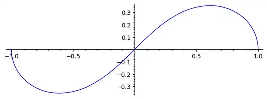
  Generated in sage via:

  var('t'); parametric_plot( ( (t+t^3)/(1+t^4), (t-t^3)/(1+t^4) ), (t, -1, 1) )
  

  The length $\varpi$, defined using the lemniscate, is the length of this parametrized curve $t\to (x(t),y(t))$: $$ \small \begin{aligned} \varpi &=\int_{-1}^1\|(x'(t),y'(t)\|\;dt = \int_{-1}^1\left\| \ \frac{( 1 - 4t^2 + t^4 )(1 + t^2)} {(1+t^4)^2} \ ,\ \frac{( 1 + 4t^2 + t^4 )(1 - t^2)} {(1+t^4)^2} \ \right\| \; dt \\ &= \int_{-1}^1 \left(\ ( 1 + 4t^2 + t^4 )^2(1 - t^2)^2 + ( 1 + 4t^2 + t^4 )^2(1 - t^2)^2 \ \right)^{1/2} \;\frac{dt}{(1+t^4)^2} \\ &= \int_{-1}^1 \left(\ \begin{array}{c} (t^{12} + 6t^{10} + 3t^8 - 20t^6 + 3t^4 + 6t^2 + 1) \\ + \\ (t^{12} - 6t^{10} + 3t^8 + 20t^6 + 3t^4 - 6t^2 + 1) \end{array} \ \right)^{1/2} \;\frac{dt}{(1+t^4)^2} \\ &= \int_{-1}^1 \left(\ 2(t^{12} + 3t^8 + 3t^4 + 1) \ \right)^{1/2} \;\frac{dt}{(1+t^4)^2} = \int_{-1}^1 \left(\ 2(t^4 + 1)^3 \ \right)^{1/2} \;\frac{dt}{(1+t^4)^2} = \sqrt 2\int_{-1}^1\frac{dt}{\sqrt{1+t^4}} \\ &= 2\sqrt 2\int_0^1\frac{dt}{\sqrt{1+t^4}} \\ &= 2\sqrt 2\int_1^\infty\frac{dt}{\sqrt{1+t^4}}\qquad \text{(using the substitution $t\to \frac 1t$)} \\ &= \sqrt 2\int_0^\infty\frac{dt}{\sqrt{1+t^4}}\qquad \text{(and using now $s=t^4$, $t=s^{1/4}$, $dt=\frac 14s^{3/4}$)} \\ &= \frac{\sqrt 2}4\int_0^\infty\frac{s^{3/4}}{(1+s)^{1/2}}\;dt = \frac{\sqrt 2}4\int_0^\infty\frac{s^{\frac14-1}}{(1+s)^{\frac 14+\frac 14}}\;dt \\ &\overset{\boldsymbol{\color{red}*}}=\frac{\sqrt 2}4 \color{blue}{B\left(\frac 14,\frac 14\right)} =2\int_0^1 \frac {du}{\sqrt{1-u^4}}\ . \\[3mm] &\qquad\text{ At ${\boldsymbol{\color{red}*}}$ we used the integral form for the Beta function $B$ with $m=n=\frac 14$:} \\ B(m,n)&:= \int_0^1 x^{m-1}x^{n-1}\; dx \qquad\text{ (using $x=\frac s{1+s}=1-\frac 1{1+s}$, $dx=\frac {ds}{(1+s)^2}$}) \\ &= \int_0^\infty \frac{s^{m-1}}{(1+s)^{m-1}} \cdot \frac 1{(1+s)^{n-1}} \cdot \frac {ds}{(1+s)^2} = \int_0^\infty \frac{s^{m-1}}{(1+s)^{m+n}} \; ds \ . \end{aligned} $$

• Above we have finally connected $\varpi$ with the AGM-integral $\int_0^1 \frac {du}{\sqrt{1-u^4}}$ via $\color{blue}{B\left(\frac 14,\frac 14\right)} $. This is one among many relations in the chain of possible equivalent forms for $\varpi$. We could stop here, because $(*)$ is holding. But there is one more important connection to an elliptic curve, that may be of interest.

• The related elliptic curve $E$ is (in affine shape) $$E\ :\qquad y^2=x^3-x\ ,$$ and need to join the integral of $1/\sqrt{1-t^4}$ on $[0,1]$ with the integral of the invariant differential $dx/y$ on this elliptic curve between the points with $x=1$ and $x=\infty$ (which make sense after passing from the affine world to the projective world), this is done by the substitution $x=1/t^2$, $dx=-2\cdot\frac1{t^3}\; dt$, $$ \small \int_{x=1}^{x=\infty} \frac{dx}{y} = \int_1^\infty\frac{dx}{\sqrt{x^3-x}} = 2 \int_0^1 \frac{dt}{t^3\cdot\sqrt{t^{-6}-t^{-2}}} = 2 \int_0^1 \frac{dt}{\sqrt{t^6(t^{-6}-t^{-2})}} =\\ 2 \int_0^1 \frac{dt}{\sqrt{1-t^4}}=\varpi \ . $$ For the elliptic curve $E$ the associated lattice has the periods $2\varpi$ and $2\varpi\cdot i$. The following sage code gives numeric support for this:

  sage: E = EllipticCurve(QQ, [-1, 0])
  sage: E
  Elliptic Curve defined by y^2 = x^3 - x over Rational Field
  sage: L = E.period_lattice()
  sage: L.0
  2.62205755429212
  sage: L.1
  2.62205755429212*I
  sage: var('t');
  sage: 2*integral( 1/sqrt(1-t^4), t, 0, 1 ).n()
  2.62205755429212
  

• Later EDIT: Above we have an explicit connection between the two integrals $\int_0^1\frac{dt}{\sqrt{1-t^4}}$ and $\int_1^\infty\frac{dx}{\sqrt{x^3-x}}$. Both integrals are mentioned in the chain of possible equivalent forms for $\varpi$. Both integrals make it possible to see the integral as an integral on an algebraic object, which is an elliptic curve. I will say something more to the last integral involving $dx$. It is hard here to give in a few words an introduction to the reach structure related to an elliptic curve, but i am trying to mention without proof a web of specific mathematical instances that make this object an interesting object to study. In the last integral we formally write $y$ for the denominator, $y=\sqrt{x^3-x}$. Squaring leads to the algebraic equation of an affine curve in Weierstraß form,$$E\ :\qquad y^2 =x^3-x\ .$$This is the curve

  sage: E = EllipticCurve(QQ, [-1, 0])
  sage: E.label()
  '32a2'  
  

  with the human label 32a2, and we can take a closer look at it on the LMFDB page, after a search of this label. On the subpage LMFDB - elliptic curves we type this label into the corresponding field, and we are linked to www.lmfdb.org/EllipticCurve/Q/32a2. At one place there is listed the real period, $\Omega$, which is $2\varpi$ on this page, by the used convention. It has two real components, which is the reason for the inserted factor two. In a picture:

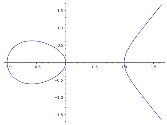  $y^2=x^3-x$" />

  Now why is this object interesting (from an arithmetic point of view)? It is so because $E$, more exactly its projective/homogenized version $Y^2Z=X^3-XZ^2$ which also contains the infinity point $\infty=O=[X_\infty:Y_\infty:Z_\infty]=[0:1:0]$, comes with a reach structure, its algebraic (and/or real and/or complex) points can be added, so we have an algebraic group $(E(\Bbb C),\oplus)$ with an addition operation $\oplus$ which is defined algebraically (i.e. using fractions of polynomials in $x,y$ in a generic case). For instance, for each point $T=(x_T,0)$ in the list $(0,0)$, $(1,0)$, $(-1,0)$, we have $T\oplus T=O$. (The infinity point $O$ is the neutral element w.r.t. $\oplus$, the three $T$-points are the two-torsion points. Counting also $O$ as torsion point we have in total four torsion points.) There is a lot of information of the elliptic curve regarding its arithmetic, and we are performing the following game. As it comes, the curve $E$ is defined over $\Bbb Q$, in fact we have a model of it over the integers, its coefficients in the polynomial equation $y^2-x^3+x=0$ are all integers. We can now "break" the $\Bbb Z$-information into pieces, we possibly lose something, but we do so. Let us consider this equation modulo some prime $p$ and "count points" modulo $p$, i.e. over the field $\Bbb F_p$, in the projective space, so we count also a point at infinity $O=\infty$. For instance, modulo five we have the eight points: $O=\infty$, $(0,0)$, $(\pm1,0)$, $(2,\pm 1)$, $(3,\pm 2)$. We now "compare" them with the number of points of the projective space $\Bbb P^1$, there are $5+1=6$ points. It turns out (by a theorem of Hasse) that the difference is "controlled". For the prime $5$ it is $a_5=\#\Bbb P^1(\Bbb F_5)-\#E(\Bbb F_5)=6-8=-2$. In a similar manner we compute: $$ \small \begin{aligned} a_3 &= \#\Bbb P^1(\Bbb F_3) -\#E(\Bbb F_3 )=4-4=0\ ,\\ a_5 &= \#\Bbb P^1(\Bbb F_5) -\#E(\Bbb F_5 )=6-8=-2\ ,\\ a_7 &= \#\Bbb P^1(\Bbb F_7) -\#E(\Bbb F_7 )=8-8=0\ ,\\ a_{11} &= \#\Bbb P^1(\Bbb F_{11})-\#E(\Bbb F_{11})=12-12=0\ ,\\ a_{13} &= \#\Bbb P^1(\Bbb F_{13})-\#E(\Bbb F_{13})=14-8=6\ ,\\ a_{17} &= \#\Bbb P^1(\Bbb F_{17})-\#E(\Bbb F_{17})=18-16=2\ ,\\ a_{19} &= \#\Bbb P^1(\Bbb F_{19})-\#E(\Bbb F_{19})=20-20=0\ ,\\ a_{23} &= \#\Bbb P^1(\Bbb F_{23})-\#E(\Bbb F_{23})=24-24=0\ ,\\ a_{29} &= \#\Bbb P^1(\Bbb F_{29})-\#E(\Bbb F_{29})=30-40=-10\ ,\\ a_{31} &= \#\Bbb P^1(\Bbb F_{31})-\#E(\Bbb F_{31})=32-32=0\ ,\\ &\ \vdots \end{aligned} $$and so on. (Compare with the coefficients of the form $q^p$ of the associated modular form.) These numbers $(a_p)$ carry the main arithmetic information in the "broken pieces" of filtering the integers through a prime numbers sieve, and in a similar manner to the construction of the Euler product for the Riemann zeta function, we can assemble the $(a_p)$ sequence into a similar product, see also the B-SD section on a page: $$ \small L(E,s)= \frac 1{1+3^{1-2s}}\cdot \frac 1{1+2\cdot 5^{-s}+5^{1-2s}}\cdot \frac 1{1+7^{1-2s}}\cdot \frac 1{1+11^{1-2s}}\cdot \frac 1{1-6\cdot 13^{-s}+13^{1-2s}}\cdot \dots $$ We formally compute this $L$-series in $s=1$, and put together in a product the information from the prime places, $$ \small \begin{aligned} L(E,1)&= \frac 3{\#E(\Bbb F_{3})}\cdot \frac 5{\#E(\Bbb F_{5})}\cdot \frac 7{\#E(\Bbb F_{7})}\cdot \frac {11}{\#E(\Bbb F_{11})}\cdot \frac {13}{\#E(\Bbb F_{13})}\cdot \frac {17}{\#E(\Bbb F_{17})}\cdot \frac {19}{\#E(\Bbb F_{19})}\cdot %\frac {23}{\#E(\Bbb F_{23})}\cdot %\frac {29}{\#E(\Bbb F_{29})}\cdot %\frac {31}{\#E(\Bbb F_{31})}\cdot \;\dots \\ &= \frac{3}{4}\cdot \frac{5}{8}\cdot \frac{7}{8}\cdot \frac{11}{12}\cdot \frac{13}{8}\cdot \frac{17}{16}\cdot \frac{19}{20}\cdot \frac{23}{24}\cdot \frac{29}{40}\cdot \frac{31}{32}\cdot \frac{37}{40}\cdot \frac{41}{32}\cdot \frac{43}{44}\cdot \frac{47}{48}\cdot \frac{53}{40}\cdot \frac{59}{60}\cdot \frac{61}{72}\cdot %\frac{67}{68}\cdot %\frac{71}{72}\cdot %\frac{73}{80}\cdot %\frac{79}{80}\cdot \;\dots \\ &\overset !=\frac{1\cdot2\varpi\cdot 1\cdot 2}{4^2} = \bbox[lightyellow]{\frac{\varpi}4} \approx0.65551438857302995261620989747277985342068\dots\ . \end{aligned} $$(The prime number two is "somehow different" in the context, the curve $E$ "degenerates" modulo two, and it turns out that there is "no" $2$-$L$-series factor.) For short, the broken arithmetic information is recollected in an expression featuring two "analytic pieces", the period $\Omega=2\varpi$, and the regulator $\operatorname{Reg}(E)=1$, together with some "global arithmetic information", which finally produces the factor $\frac 2{4^2}$. (The $4$ is the number of torsion points.)

  In my eyes, this connection of an elliptic integral with the (real) period of an elliptic curve, is the most intricate and intriguing instance of a transcendent number in a situation governed by an algebraic situation.

  The above $\overset!=$ is an equality, it is a theorem.

  But we have no similar information for the "cousin" elliptic curve $y^2=x^3-226x$ with real period $\int_{\sqrt{226}}^\infty\frac{dx}{x^3-226x}=\bbox[lightyellow]{\frac{\varpi}{\sqrt[4]{226}}}$. Of course, the complication is on the arithmetic side, this is an elliptic curve over $\Bbb Q$ with two torsion points, $O=\infty$ and $(0,0)$, rank three, generators of the free part of $E(\Bbb Q)$ being $(-1,15)$, $(-8,36)$, $(121/4, 1155/8)$, and regulator $\operatorname{Reg}(E)\approx 23.6131617974\dots$ computed from them. Then any progress in showing the B-SD relation: $$ \small \frac{L'''(E,1)}{3!} \overset? = \frac 1{2^2}\cdot1\cdot\frac{2\varpi}{\sqrt[4]{226}}\cdot \operatorname{Reg}(E)\cdot(226^2) $$ would be a true breakthrough. I have to stop here.

Answer 3

Definition

Let $0<a<b.$ Set $a_0=a,b_0=b$ and $a_n=\sqrt{a_{n-1}b_{n-1}}, b_n=\frac{a_{n-1}+b_{n-1}}2$ for $n\geq1.$ Then, $a_n$ $(b_n)$ is an increasing (a decreasing) bounded sequence with $a_n<b_n$. So they are convergent with equal limits. We define the arithmetic-geometric mean of $a$ and $b$ as $$AMG(a,b)=b_\infty=a_\infty.$$

Definition $$I(a,b)=\int_0^{\frac{\pi}2}\frac{d\theta}{\sqrt{a^2\cos^2\theta+b^2\sin^2\theta}}$$ Notice that $$I(a,a)=\frac{\pi}{2a}\tag{1a}$$ and that $$I(a,b)=\frac1a K\left(\sqrt{1-\frac{b^2}{a^2}}\right)\tag{1b}$$ where $K(k)$ is the complete elliptic integral of the first kind.

Landen Transformation

$$I(u,v)=I\left(\sqrt{uv},\frac{u+v}2\right)\tag2 $$

Results

Using $(2)$ repeatedly and $(1a)$, $$AMG(a,b)=\frac{\pi}{2I(a,b)}\tag{3a}$$ and then by $(1b)$ $$AMG(a,b)=\frac{a\pi}{2K \left( \sqrt{1-\frac{b^2}{a^2}}\right)} \tag{3b}$$

Application

Put $a=1,b=\sqrt2$ in $(3b)$: $$AMG\left(1,\sqrt2\right)=\frac{\pi}{2K(i)}=\frac{\pi}{\varpi}$$ since $$K(i)=\int_0^{\frac{\pi}{2}}\frac{d\theta}{\sqrt{1-i^2\sin^2\theta}}= \int_0^{\frac{\pi}{2}}\frac{d\theta}{\sqrt{1+\sin^2\theta}} \stackrel{\sin\theta=t}{=}\int_0^1\frac{dt}{\sqrt{1-t^4}}=\frac{\varpi}2 $$ quarter length of the lemniscate.