Proof that a moment generating function is unique

Question

I am trying to understand the proof behind why the Moment Generating Function (https://en.wikipedia.org/wiki/Moment-generating_function) of a random variable is is unique.

For example, consider the following case of two random variables $X$ and $Y$, i.e both random variables are in terms of $x$, e.g. $x = f(x)$, $y = g(x)$:

$$ \text{PDF of } X: \quad f(x) $$

$$ \text{PDF of } Y: \quad f(y) $$

$$ M_X(t) = \mathbb{E}[e^{tX}] = \int_{-\infty}^{\infty} e^{tx} f(x) \, dx $$

$$ M_Y(t) = \mathbb{E}[e^{tY}] = \int_{-\infty}^{\infty} e^{ty} f(y) \, dx $$

From here, define a function that is the difference between both PDF's : $d(x) = f(x) - f(y)$

Using this, we can also define a function which is the difference between both MGF's:

$$ Z = M_X(t) - M_Y(t) = \int_{-\infty}^{\infty} e^{tx} f(x) \, dx - \int_{-\infty}^{\infty} e^{ty} f(y) \, dy $$

$$ = \int_{-\infty}^{\infty} \left [ e^{tx} f(x) - e^{ty} f(y) \right ] \, dx $$

$$ = \int_{-\infty}^{\infty} e^{tx} \left[ f(x) - f(y) \right ] \, dx $$

$$ = \int_{-\infty}^{\infty} e^{tx} \, d(x) \, dx $$

Now, consider the following:

$$ \text{Case 1:} \quad d(x) = f(x) - f(y) = c_1 \quad \text{where} \quad c_1 > 0 \quad \text{and} \quad c_1 \neq 0 $$

$$ \text{Case 2:} \quad d(x) = f(x) - f(y) = c_2 \quad \text{where} \quad c_2 > 0 \quad \text{and} \quad c_2 \neq 0 $$

The implications of both cases are:

$$ \text{Case 1:} \quad Z = \int_{-\infty}^{\infty} e^{tx} c_1 dx = z_1 $$

$$ \text{Case 2:} \quad Z = \int_{-\infty}^{\infty} e^{tx} c_2 dx = z_2 $$

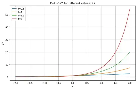
Now, when we look at the graph for $e^{tx}$, we can see that when $t>0$, the function is always positive and increasing (monotonic):

This means that the integral of $e^{tx}$ by itself must always be greater than $0$.

This is where I use proof by contradiction:

• Let's suppose that Case 1 is $0$, i.e. $z_1 = 0$
• If Case 1 is $0$, this means that Case 2 $\neq 0$.
• This is because the function $e^{tx}$ is always increasing by itself, and case 2 is pushing the function further than case 1

Thus, if we need $Z$ (difference between two MGFs) to always be $0$, then $f(x)$ always has to be equal to $f(y)$ - implying the uniqueness of MGFs.

Is my proof correct?

---

# plot 1
import numpy as np
import matplotlib.pyplot as plt
x = np.linspace(-2, 2, 400)
t_values = [0.5, 1, 1.5, 2]
plt.figure(figsize=(10, 6))
for t in t_values:
    y = np.exp(t * x)
    plt.plot(x, y, label=f't={t}')
plt.title('Plot of $e^{tx}$ for different values of $t$')
plt.xlabel('$x$')
plt.ylabel('$e^{tx}$')
plt.legend()
plt.grid(True)
plt.show()
plot 2
import numpy as np
import matplotlib.pyplot as plt
x = np.linspace(-2, 2, 400)
t = 1
c_values = [0.5, 1, 1.5, 2]
plt.figure(figsize=(10, 6))
for c in c_values:
    y = c * np.exp(t * x)
    plt.plot(x, y, label=f'c={c}')
plt.title('Plot of $c \cdot e^{tx}$ for different values of $c$ with $t$ fixed')
plt.xlabel('$x$')
plt.ylabel('$c \cdot e^{tx}$')
plt.legend()
plt.grid(True)
plt.show()
#plot 3
import numpy as np
import matplotlib.pyplot as plt
from scipy.integrate import quad
x = np.linspace(0, 2, 400)
t = 1
c_values = [0.5, 1, 1.5, 2]
def integrand(x, c, t):
    return c * np.exp(t * x)
cumulative_integrals = np.zeros_like(x)
for c in c_values:
    integral_values = [quad(integrand, 0, xi, args=(c, t))[0] for xi in x]
    cumulative_integrals += integral_values
    plt.fill_between(x, cumulative_integrals - integral_values, cumulative_integrals, label=f'c={c}')
plt.title('Cumulative Integrals of $c \cdot e^{tx}$ from 0 to 2 for different values of $c$ with $t$ fixed')
plt.xlabel('$x$')
plt.ylabel('Cumulative Integral Value')
plt.legend()
plt.grid(True)
plt.show()

Answer 1

Your proof is not correct.

What you want to show is if $M_X(t)=M_Y(t)$ then $F_X(x)=F_Y(x)$. In fact, in your attempt, you are assuming that the density function exists and they can be written as $f_X(x)$ and $f_Y(x)$, note that for a function, the argument input is just a notation, it is better to label/index your function using the corresponding random variable. However, note that two different density function that differ by a set of measure zero can give you the same CDF, thus, when we compare density functions, you might like to compare equality almost everywhere and not identical everywhere.

Let's compute the difference of $M_X(t)$ and $M_Y(t)$, the quantity that is denoted by $Z$.

\begin{align}Z(t)&=M_X(t)-M_Y(t)\\&=\mathbb{E}[\exp(tX)]-\mathbb{E}[\exp(tY)] \\ &=\int_{-\infty}^{\infty} \exp(tx) f_X(x) - \exp(tx) f_Y(x) \, dx \\ &=\int_{-\infty}^\infty \exp(tx) d(x) \, dx \end{align}

Now, the main confusing part is the following:

• Why do you consider two values? $c_1 $ and $c_2$, are these both positive constants? do they only take two values? If two functions are different, they should be able to take different values at many locations. The assumption is not valid.
• Also, $Z$ should be a function of $t$.

If $Z(t)$ is zero, now the question is must $d$ be identically $0$ everywhere? or can it take some positive values and some negative values and they cancel out?

With all these points raised, we can see that the proof attempt doesn't answer most of these points.

This is an inversion problem, given that $Z(t)$ is zero, can we show that $d$ is zero almost everywhere?

I encourage you to refer to the solutions posted here. In particular, the special case where the supports are discrete and finite.