Note: My answer and code differs from yours by a transposition. That is, if we are in $\mathbb{R}^d$ and I have $n$ vectors $X_1,\ldots,X_n\in\mathbb{R}^d$, then those are arranged in the columns of my matrix $X \in\mathbb{R}^{n\times d}$:
$$X = \begin{bmatrix} | & & | \\ X_1 & \ldots & X_n \\ | & & | \end{bmatrix}, \quad X^T = \begin{bmatrix} - X_1^T - \\ \vdots \\ - X_n^T - \end{bmatrix}.$$
So my $X^T\in\mathbb{R}^{n\times d}$ (XT in my code) is your $X$.
Also, since the constraint $(Y^TY)_{ii} = 1$ is automatically satisfied I do not discuss it below. You can take non-normalized vectors if you wished, and the below method would reconstruct those.
The Gramian
You are given the matrix of dot products (the Gramian):
$$G =
\begin{bmatrix}
X_1 \cdot X_1 & \ldots & X_1 \cdot X_n \\
\vdots & & \vdots \\
X_n \cdot X_1 & \ldots & X_n \cdot X_n
\end{bmatrix}
=
\begin{bmatrix}
X_1^T X_1 & \ldots & X_1^T X_n \\
\vdots & & \vdots \\
X_n^TX_1 & \ldots & X_n^T X_n
\end{bmatrix} = X^TX \in \mathbb{R}^{n\times n}.$$
The matrix is symmetric $G^T = (X^TX)^T = X^T(X^T)^T = X^TX = G$, and positive semi-definite $u^TGu = u^TX^TXu = (Xu)^T(Xu) = \|Xu\|^2_2\geq 0$. The matrix is positive definite iff the vectors $X_1,\ldots,X_n$ are linearly independent. A necessary but insufficient conditions for this is that $n\leq d$.
Since $G$ is real symmetric it admits an eigendecomposition $G=WDW^T$ where the eigenvectors are orthonormal $W\in O(n) = \{Q\in\mathbb{R}^{n\times n}\,:\, W^TW=WW^T=I_n\}$, and the eigenvalues are real $D\in\mathbb{R}^{n\times n}$. Since $G$ is positive semi-definite, the eigenvalues $D_{ii}$ are additionally non-negative.
Case 1: $n=d$
Suppose that $n= d$ then:
$$G=WDW^T \stackrel{(i)}{=} W\underbrace{\sqrt{D}}_{\sqrt{D}\in\mathbb{R}^{n\times n}}\sqrt{D}^TW^T = \underbrace{(W\sqrt{D})}_{\tilde{Y}^T\in\mathbb{R}^{n\times n}}\underbrace{(W\sqrt{D})^T}_{\tilde{Y}\in\mathbb{R}^{n\times n}} =
\tilde{Y}^T\tilde{Y}.$$
$(i)$ Since $D_{ii}\geq 0$ it follows $\sqrt{D_{ii}}\in\mathbb{R}$ and thus
$\sqrt{D}\in\mathbb{R}^{n\times n}$ and $\tilde{Y}\in\mathbb{R}^{n\times n}$. If that was not the case the matrix $\tilde{Y}$ could have become complex-valued. Since $\tilde{Y}$ is of the desired size, we can just use $Y=\tilde{Y}$ as the reconstructed vectors.
Note that this is not the only solution, and for any $Q\in O(d)$ we have that $Y_Q = QY$ is also a solution, since
$$Y_Q^TY_Q = (QY)^T(QY) = Y^T\underbrace{Q^TQ}_{I}Y = Y^TY = G.$$
Case 2: $n<d$
In the case $n<d$ our Gramian is only $n\times n$ and the resulting $Y$ is also $n\times n$, but we need $d$-dimensional vectors. We could arbitrarily choose an $n$-dimensional subspace of $\mathbb{R}^d$ and situate the solution there. A simple subspace is the one where the last coordinates are zero: $x_i=0$ for $n+1\leq i \leq d$. Then we just need to extend the matrix with $(d-n)$ additional rows of zeros:
$$Y = \begin{bmatrix} \tilde{Y} \\ 0_{(n-d)\times n}\end{bmatrix} \in\mathbb{R}^{d\times n}.$$
In my code down below the adjust_matrix function performs this padding if $n<d$ (but it performs it on $\tilde{Y}^T$).
As before, the solution is not unique and any $Y_Q = QY$ is also a solution.
Case 3: $d<n$
The case $d<n$ is arguably the most interesting one in practice. The rank of the matrix can be at most $d<n$, which automatically means that it is singular. It also means that there are at most $d$ non-zero eigenvalues. Let the eigenvalues in the eigendecomposition be ordered from largest to smallest, then the non-zero eigenvalues are in the upper left block of $D$:
\begin{align*}
G&=WDW^T \\
&=
\begin{bmatrix}
| & & | & | & & | \\
W_1 & \ldots & W_d & W_{d+1} & \ldots & W_n \\
| & & | & | & & |
\end{bmatrix}
\begin{bmatrix}
\sqrt{D_{11}}^2 & & & & & \\
& \ddots & & & & \\
& & \sqrt{D_{dd}}^2 & & & \\
& & & 0 & & \\
& & & & \ddots & \\
& & & & & 0
\end{bmatrix}W^T \\
&= \underbrace{\begin{bmatrix}
| & & | & | & & | \\
W_1\sqrt{D_{11}} & \ldots & W_d\sqrt{D_{dd}} & 0 & \ldots & 0 \\
| & & | & | & & |
\end{bmatrix}}_{\tilde{Y}^T=W\sqrt{D}\in\mathbb{R}^{n\times n}}
\underbrace{\begin{bmatrix}
- \sqrt{D_{11}}W_1^T - \\
\vdots \\
-\sqrt{D_{dd}}W_d^T - \\
- 0^T - \\
\vdots \\
- 0^T -
\end{bmatrix}}_{\tilde{Y}=(W\sqrt{D})^T\in\mathbb{R}^{n\times n}}
\\
&= \underbrace{\begin{bmatrix}
| & & | \\
W_1\sqrt{D_{11}} & \ldots & W_d\sqrt{D_{dd}} \\
| & & |
\end{bmatrix}}_{Y^T\in\mathbb{R}^{n\times d}}
\underbrace{\begin{bmatrix}
- \sqrt{D_{11}}W_1^T - \\
\vdots \\
-\sqrt{D_{dd}}W_d^T -
\end{bmatrix}}_{Y\in\mathbb{R}^{d\times n}}.
\end{align*}
Note that $D_{dd}$ and lower terms can also be zero, but that is not relevant for this, the point was to reduce $\tilde{Y}\in\mathbb{R}^{n\times n}$ to $Y\in\mathbb{R}^{d\times n}$. This truncation of the matrix for $d<n$ happens in my code below through adjust_matrix. Note that knowing the number of non-zero eigenvalues $r$ may be relevant for computational efficiency though, since if you set $k=r$ instead of $k=d$ in eigsh, you only need to compute the $r$ eigenvectors and eigenvalues in that case and get a matrix of size $r\times n$. Then you can pad the matrix with zeroes to reach a dimension of $d\times n$.
As before, the solution is defined only up to an orthogonal transformation $Q\in O(d)$. This held in all cases and the extra degrees of freedom are then $\dim O(d) = d(d-1)/2$.
Number of Coefficients in $G,Q$ vs $X$
Note that the space of symmetric matrices $\operatorname{Sym}(n)$ has dimension $n(n+1)/2$ (this is referring to the data in $G$). As a sanity check, for $n=d$ we have:
$$\dim O(d) + \dim \operatorname{Sym}(n) = d(d-1)/2 + n(n+1)/2 = n^2 = nd.$$
So the amount of data in $X\in\mathbb{R}^{d\times n}$ is equivalent to the amount of data in $G$ and $Q$ for $n=d$. We can show that the same is true if $d=n+1$. If $d\not\in\{n,n+1\}$ we can show that $\dim O(d) + \dim \operatorname{Sym}(n)>nd$, i.e., if we store $Q$ and $G$ instead of $X$, that is actually more wasteful:
\begin{align*}
f(d) &= \dim O(d) + \dim \operatorname{Sym}(n) -nd = \frac{d^2}{2} - \left(n+\frac{1}{2}\right)d + \frac{n^2+n}{2}, \\
D&= \left(n+\frac{1}{2}\right)^2 - n^2-n = \frac{1}{4} \\
d_{1,2} &= n+\frac{1}{2}\pm\frac{1}{2} \in \{n, n+1\} \implies
f(d)>0 \text{ for } d\in\mathbb{N}\setminus \{n, n+1\}.
\end{align*}
Consider storing a single vector then you need to store $d$ components. On the other hand $\dim O(d)$ grows quadratically with the dimension. Vice versa, consider $d$ fixed, and grow $n$. $X$ grows linearly in $n$ while $G$ grows quadratically. So in either case you can't really use this as a compression technique, unless $d\gg n$ and you just store $G$. Although I suppose that is not what you're using this for.
How to find $Q \,:\, X = QY$
Provided you have computed $Y$ and you have $X$ you can find the $Q$ such that $X=QY$ by solving the orthogonal Procrustes problem:
$$\min_{Q\in O(d)}\|QY-X\|^2_2 \implies Q=UV^T \,:\, XY^T = USV^T.$$
That is, you can compute the SVD of $XY^T$ and drop the singular values matrix. I use this as a sanity check in my code below in order to verify that $Y$ can indeed be brought to $X$ with an orthogonal transformation of the vectors.
Computational Aspects
As you saw from the above, in all cases (regardless whether $G$ is singular) you can use the eigendecomposition in order to compute $Y$ from $G$. When $d\ll n$ this is especially efficient if you compute just the $d$ eigenvectors corresponding to the largest eigenvalues (or if you know the rank $r$ and $r<d$, you could just compute the $r$ eigenvectors), e.g. by using scipy.sparse.linalg.eigsh which calls ARPACK under the hood, and thus uses Lanczos. When $d>=n$ you can do a full eigendecomposition on the matrix $G\in\mathbb{R}^{n\times n}$ by using np.linalg.eigh. Or again, if you know that its rank is lower, you can stop at that.
When $n\leq d$ another option is to compute the square root of $G$, i.e., $Y=\sqrt{G}$ (you can use scipy.linalg.sparse.sqrtm). Note that this does not work when $n>d$ since then you cannot just drop the last $(n-d)$ columns of $\tilde{Y}$ in order to get $Y$. Also it may happen that $\sqrt{G}\in\mathbb{C}^{n\times n}$ due to numerical error. In my code I just drop the imaginary part in that scenario, but I doubt that's the most robust thing.
When $G$ is non-singular (a necessary but insufficient condition is $n=d$), you can also use the Cholesky decomposition: $G=LL^T$. Then $Y=L^T$. If $G$ is singular, you could use the $LDL^T$ decomposition. Then you could drop the rows of $L$ corresponding to zeroes in $D$ in order to get $Y$. This works also when $n>d$.
From the above methods I would expect the eigendecomposition with eigsh to be the fastest, especially for $d\ll n$. I don't know how efficient the square root and Cholesky are comparatively in python. So they may make sense for when $n$ is large and $n\approx d$, but you should profile that yourself.
Code
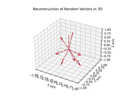
I wrote some code to demonstrate that this works (with Cholesky, the square root, LDL^T, and eigendecomposition with only $\min(n,d)$ vectors). This should work for any number of vectors $n>0$ and in whatever dimension (for the visualisation the dimension must be $2$ or $3$). You can see the result here:
The code also works when you have linearly dependent vectors: you can test the commented line XT=np.array([[1.0,0,0],[1.0,0.0,0]]).
import numpy as np
import scipy
import scipy.sparse.linalg
import matplotlib.pyplot as plt
from mpl_toolkits.mplot3d import Axes3D
generates uniformly distributed points on the unit sphere
def generate_normalized_vectors(n,d):
# Generate n normally distributed vectors in d-D
random_vectors = np.random.normal(size=(n, d))
# Normalize the vectors
norms = np.linalg.norm(random_vectors, axis=1, keepdims=True)
normalized_vectors = random_vectors / norms
return normalized_vectors
truncates the last (n-d) columns of Y^T if d<n
adds (d-n) extra zero columns to Y^T if n>d
def adjust_matrix(A, d):
n = A.shape[1] # Assuming A is a square matrix (n x n)
if d < n:
# Drop the last (n - d) columns
adjusted_A = A[:, :d]
elif d > n:
# Add (d - n) zero columns
zero_columns = np.zeros((n, d - n))
adjusted_A = np.hstack((A, zero_columns))
else:
# d == n, do nothing
adjusted_A = A
return adjusted_A
solves min_{Q^TQ = I} ||QA-B||^2_2
If BA^T = USV^T, then Q = UV^T
def procrustes(A,B):
U,S,VT = np.linalg.svd(np.matmul(B,A.T));
return np.matmul(U,VT);
def draw_vectors(XT, XT_rec):
d = XT.shape[1];
# Visualization
fig = plt.figure()
if d==2:
ax = fig.add_subplot(111)
else:
ax = fig.add_subplot(111, projection='3d')
# Plot the vectors
origin = np.zeros((d, 1)) # Origin point
for vector in XT:
if d==2:
ax.quiver(*origin, *vector,
ls='-', linewidth=1,
angles='xy', scale_units='xy', scale=1, facecolor='none', edgecolor = 'k')
else:
ax.quiver(*origin, *vector, linestyle='dashed', normalize=False)
for vector in XT_rec:
if d==2:
ax.quiver(*origin, *vector,
ls='-.', linewidth=1,
angles='xy', scale_units='xy', scale=1, facecolor='none', edgecolor='r')
else:
ax.quiver(*origin, *vector, color = 'red', linestyle='dashdot', normalize=False)
# Set limits and labels
ax.set_xlim([-1, 1])
ax.set_ylim([-1, 1])
if d==3:
ax.set_zlim([-1, 1])
ax.set_xlabel('X axis')
ax.set_ylabel('Y axis')
if d==3:
ax.set_zlabel('Z axis')
if d==2:
ax.set_title('Reconstruction of Random Vectors in 2D')
else:
ax.set_title('Reconstruction of Random Vectors in 3D')
plt.show()
number of vectors
n = 8
dimension
d = 3
0: Use Cholesky: G=LL^T -> Y^T = L (works only for n<=d and non-singular matrices)
1: Use matrix square root: Y^T = sqrt(G)=Vsqrt(D)V^T (works only for n<=d)
2: Use Bunch-Kaufman: G=LDL^T, Y^T= [L sqrt(D)]|_{nxd}
3: Use eigendecomposition: G=VDV^T -> Y^T = [V sqrt(D)]|_{nxd}
mode = 3
switch to eigendecomposition if Cholesky or sqrt were chosen but d<n
if d<n and mode<2:
if mode==0:
print("Cholesky was specified but d<n. Switching to eigendecomposition.")
else:
print("Matrix square root was specified but d<n. Switching to eigendecomposition.")
mode = 3
generate random vectors in the rows of X^T in R^{nxd}
XT = generate_normalized_vectors(n,d)
to test degernate case for n<d
#XT=np.array([[1.0,0,0],[1.0,0.0,0]])
Gram matrix G = X^TX, a R^{nxn} positive semi-definite matrix
G = np.matmul(XT,XT.T)
G=LL^T -> Y^T = [L]|_{n x d}
if mode==0:
# Use Cholesky if the matrix is non-singular (can happen only for d==n)
if n<=d and np.linalg.cond(G) < 1.0/np.finfo(G.dtype).eps:
print("Using Cholesky.")
YTnD = np.linalg.cholesky(G)
else:
print("Matrix is singular. Cannot use Choleksy. Switching to LDL^T decomposition.")
mode = 2
sqrt(G) = V sqrt(D) V^T -> Y^T = [V sqrt(D) V^T]|_{n x d}
if mode==1:
print("Using matrix square root.")
YTnD = np.real(scipy.linalg.sqrtm(G))
G=LDL^T -> Y^T = [L sqrt(D)]|_{n x d} decomposition
if mode==2:
print("Using LDL^T.")
L, D, perm = scipy.linalg.ldl(G)
# take the square root of D and drop the terms
# that are supposed to be zero
for i in range (0,min(d,n)):
D[i,i] = np.sqrt(D[i,i])
for i in range(min(d,n),n):
D[i,i] = 0
# Once we truncate L sqrt(D) we will get Y^T
YTnD = np.matmul(L, D)
G = VDV^T -> Y^T = V sqrt(D)
if mode==3:
if n<=d:
print("Using full eigendecomposition.")
D, W = np.linalg.eigh(G)
else: # d<n
print("Using partial eigendecomposition.")
D, W = scipy.sparse.linalg.eigsh(G, k=d, which='LM')
YTnD = np.matmul(W,np.diag(np.sqrt(D)));
truncate or extend as necessary the matrix from R^{nxn} to R^{nxd}
YT = adjust_matrix(YTnD, d)
reconstruct XT from YT exactly
Q = procrustes(XT.T,YT.T);
XT_rec = np.matmul(YT, Q);
draw_vectors(XT,XT_rec)
