Use of smooth bump functions in probabilities: make any sense?

Question

Use of smooth bump functions in probabilities: make any sense?

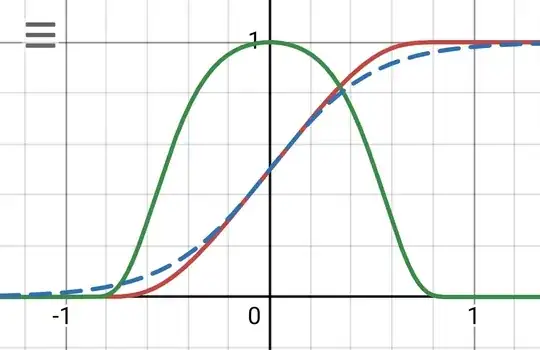
After reading this answer I started to wonder if it make sense to define a Cumulative distribution function as follows: $$F(x)=\begin{cases} \dfrac{1}{2}\left(1+\tanh\left(\dfrac{2x}{1-x^2}\right)\right),\ |x|<1\\ 0,\ x\leq -1\\ 1,\ x\geq 1\end{cases}$$ which is a smooth transition function class $C^\infty$ function, but I don't know if make sense, conceptually speaking, that before some point ($x=-1$) all probability is exactly zero, and after some point ($x=1$) all probability is exactly one.

This is better seen in its Probability density function $f(x)=F'(x)$ which is given by: $$f(x)=\begin{cases} 0,\ |x|\geq 1\\ \left(x^2+1\right)\left(\dfrac{\text{sech}\left(\frac{2x}{1-x^2}\right)}{1-x^2}\right)^2,\ |x|<1\end{cases}$$ where you could see that $f(x)\in C_c^\infty$ making it an example of a smooth bump function which have some interesting properties, like being examples of Non-analytic smooth function since at their edges they smoothly becomes a flat function, something classic powers series cannot do because of the Identity theorem. Notice that $f(x)>0,\ \forall x$ and $\int\limits_{-\infty}^{\infty} f(x)\ dx = \int\limits_{-1}^{1} f(x)\ dx =1$ as shown in the mentioned answer, so is indeed a probability density function, being defined in the whole real line (the piecewise is done such it excludes undefined points).

You can see their plots in Desmos:

Even with the mentioned weirdness of this functions, for someone with just graduated math knowledge they don't seen strange at all: as example, $F(x)$ it is just a modification of a Logistic function since: $$\dfrac{1}{2}\left(1+\tanh\left(\dfrac{2x}{1-x^2}\right)\right)=\dfrac{1}{1+\exp\left(\frac{-4x}{1-x^2}\right)}$$

where in the blue dashed line it is compared to the logistic function: $$L(x)=\dfrac{1}{1+e^{-4x}}$$

and they look quite similar, with the exception that the derivative of $F(x)$ is compact-supported.

Even so, looking the Wikipedia for the Logistic regression, the logistic function could be used as for Binary classification or as an activation function for artificial neuronal networks, but it don't appears as any of the examples, even so just recently it was added as example of a Sigmoid function in Wikipedia.

So given that it looks inoffensive, it lack of pressence in Wikipedia makes me wonder if there are some fundamental issues that make it undesirable as a CDF, or as Logistic regression fit or neuronal activation function (somehow all are related).

---

Added later

After the answer somehow right, but not directly answering the question, I want to reframe it:

Imagine the following thought experiment:

I have a squared section of 2x2 meters (units are irrelevant here) aligned with the cartesian coordinate system with the center of the square at the point $(x,\ y)=(0,\ 0)$.

In this square, I am able to measure only the $x$ coordinate of water drops that fall into the square from a circular aperture of radius $1/2$ meters located over the square at some height (lets say 1 meter), such as the center of the circular aperture is located also at at the point $(x,\ y)=(0,\ 0)$.

The water drops fall over the circular aperture randomly following a uniform distribution, so I am expecting, here inaccurately, to have some concentration of points near the center of the $x$ axis, thinking in how the Box–Muller transform builts a Gaussian distribution as the $x$ axis of a 2D uniformly distributed variable in polar form, but also accurately given the concentration inequalities.

As observer, I have only access to the data points of the water drops in the x-axis, so I have no clue from where the drops are falling (don't know the height, the aperture shape, neither the falling distribution before the aperture).

Now imagine the data is such, that it could be modeled through the following fitting distribution functions: $f_i(x)= c_i \hat{f}_i(x)$ where $c_i$ are normalizing constants and the shape functions $\hat{f}_i(x)$ are given by:

1. A gaussian shape $$\hat{f}_1(x)=e^{-16x^2}$$
2. A compact-supported polynomial $$\hat{f}_2(x)=\left(\frac{1-4x^2+|1-4x^2|}{2}\right)^4$$
3. A compact-supported trigonometric function $$\hat{f}_3(x)=\cos^4(\pi x)\ \theta(1-4x^2)$$ with $\theta(x)$ the heaviside step function.
4. A smooth compact-supported function $$\hat{f}_4(x)= e^{-\frac{1}{\left(x+\frac12\right)\left(\frac12-x\right)}}\ e^{\frac{1}{\left(\frac{1}{2}\right)^2}}$$

all of them could been seen here:

Also assume that from the data I cannot dismiss any of these curves because of p-values or significance of the confidence intervals (or other classic curve fitting figures).

Postulate 1: From what I know of the data I see, I should dismiss the Gaussian envelope $\hat{f}_1(x)$ since I know beforehand I will only have data points strictly among $[-1,\ 1]$, so I will pick only compact-supported alternatives (maybe this postulate is mistaken, but I am using it here for developing what I would ask next).

In the same sense, Are there any reasons why I should pick the smooth alternative as the representative model for the data?

Answer 1

There's a common misconception that parametric probability distributions arise because of a need to model data that appears to satisfy certain shape criteria--e.g., data that have a "bell-shaped" frequency should be modeled by a normal distribution. This is incorrect.

Most if not all distributions used in statistical practice arise from the investigation of the mathematical properties of particular random phenomena under various assumptions. The normal distribution arises from the central limit theorem. The binomial distribution is the sum of iid Bernoulli variates. The geometric distribution is a discrete stopping time distribution; etc. Their functional forms look the way they do because some underlying behavior is being modeled, not because we need the curve to look a particular way.

So, as to why such a CDF is "undesirable," that's not really the relevant question. Rather, the question should be, "what random process or property exists that would give rise to such a parametric model?" This is what makes parametric distributions useful--their relationship to the process that generates data.

Answer 2

As far as statistical modelling is concerned:

1. This is a valid statistical model. This is a not a high-bar to pass. Any family of probability distributions is going to be a valid statistical model.

2. This model makes a very specific prediction for the data: that the probability tends aggressively fast to 0 at the limits of the support. To me, that's a disqualifying flaw for this model, and any smooth bump model. Depending on how the model is fitted, this might be gigantic issue or a minor issue.