4

The cumulative distribution function of the standard normal distribution $\Phi(z)=\displaystyle\frac{1}{\sqrt{2\pi}}\int_{-\infty}^z e^{-t^2/2}dt$ cannot be expressed in terms of elementary functions, thus computing values is subject of numerical approximations (or iterating converging series up to a reasonable limit). Ditto for the inverse of it, quantile function or probit, $\text{probit}(\Phi(z))=\Phi^{-1}(\Phi(z))=z$. While there exist approximations for the later it may also be set up as root finding procedure for $\Phi^{-1}(\Phi(z))-z=0$.
A look at the plot of the probit function...
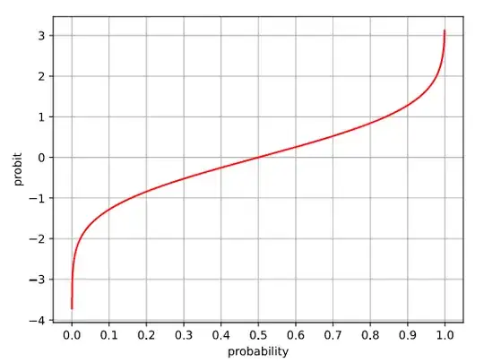
The probit is the quantile function of the normal distribution (source: Wikipedia)
... shows from $\Phi(z)=0.1$ to $0.9$ roughly a straight line. In this section Newton's method works perfectly. In contrast for the lower and upper ends an alternate root finder is more apt.
"Algorithm 39", Areas Under The Normal Curve, uses as approximation for the tails $\Phi(z)\approx\displaystyle\frac{1}{\sqrt{2\pi}}\exp\left (-\frac{z^2}{2}\right )\cdot f(z)$ where $f$ is a rational function.

Question: Which root finder would be the best for the outer sections of this approximation?

Short clarification: The question is not how to put on a procedure with erfc to compute $\Phi^{-1}$, I'm looking for an adequate root finder using a. m. "Algorithm 39".

Long clarification: "Algorithm 39" was published in 1969 when computing power was valuable enough to justify some effort in devising fast approaches, which comprises also the preparation of an iteration. So my query is, at that time, which algorithm based on "Algorithm 39" would work best for computing the quantile function's tails (that is $\Phi(z)$ above 0.9 and below 0.1)?
"Algorithm 39" computes for $z\ge 1.28$ $$\Phi(z)\approx\displaystyle\frac{p\cdot e^{\displaystyle -z^2/2}}{z+q+r}\ \ \ \text{with}\ r=\cfrac{b_1}{z+b_2+\cfrac{b_3}{z+b_4+\cfrac{b_5}{z+b_6+\cfrac{b_7}{z+b_8+\cfrac{b_9}{z+b_{10}}}}}}$$ and
$p=0.398942280385,\ q=-3.8052\cdot 10^{-8},\ b_1=1.00000615302,\ b_2=0.000398064794,\\\ b_3=1.98615381364,\ b_4=-0.151679116635,\ b_5=5.29330324926,\ b_6=4.8385912808,\\\ b_7=-15.1508972451,\ b_8=0.742380924027,\ b_9=30.789933034,\ b_{10}=3.99019417011$

What I found so far: not too much. While root-finder of higher-order (higher than Newton’s method) may work (iff the initial iteration value $x_0$ ensures $f(x_i) = 0$ to be an attractor), it might be overdone somehow when 10..12 digits accuracy is sufficient.

Playing a bit with the quantile or probit function $\Phi^{-1}(p)$ with $p\lt 0.1$, which when approaching $0$ is "diving down" quite fast (see diagram above), I found some "linearisation" (not in the mathematical sense) by conversion $y=\exp(-(\Phi^{-1}(p))^2/2)$, see (and compare with the plot above): converted Phi^-1 This leads to ...
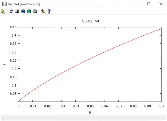
Additional questions: Could this conversion be helpful for computing $\Phi^{-1}$ by root-finding? How might an adequate iterative function look like? Are there examples which use a similar conversion to ease root-finding?

m-stgt
  • 575

1 Answers1

6

Many standard math libraries (e.g. C99, C++11,Fortran 2008) offer implementations of the complementary error function $\mathrm{erfc}$ making it worthwhile to take a detour through that. If we let $\mathrm{normcdfinv}()$ represent the inverse of the CDF of the normal distribution, and $\mathrm{erfcinv}()$ the inverse of the complementary error function, then $\mathrm{normcdfinv}(a) = -\sqrt{2} \ \mathrm{erfcinv} (2a)$.

The inverse of the complementary error function lends itself to root finding by Halley iteration:

$$x_{i+1}=x_{i}-\frac{f(x_{i})}{f'(x_{i})}\left[1-\frac{f(x_{i})}{f'(x_{i})} \cdot\frac{f''(x_{i})}{2f'(x_{i})} \right]^{-1}$$

With $f(x)=\mathrm{erfc}(x)-y$, we have $\frac{f(x_{i})}{f'(x_{i})} = -\frac{1}{2}\sqrt{\pi}\exp(x^2)(\mathrm{erfc}(x_{i}) - y)$ and $\frac{f''(x_{i})}{2f'(x_{i})}=-x_{i}$. Given $y$, a simple starting guess would be $x_{0} = \sqrt{-\ln{y}}$. The complete setup becomes:

$c := -\frac{1}{2}\sqrt {\pi}$
$f := y \gt 1$
$\mathrm{if} \ \ (f) \ \ \mathrm{then} \ \ y := 2 - y$
$x_{0} := \sqrt{-\ln{y}}$

Now iterate for as long as necessary:

$u_{i} := c \cdot \exp (x_{i}^{2}) \cdot (\mathrm{erfc}(x_{i}) - y) \\ d_{i} := \dfrac{u_{i}}{1 + x_{i} \cdot u_{i}} \\ x_{i+1} := x_{i} - d_{i}$

We need to apply a final fix-up based on the original argument transformation:

$\mathrm{erfcinv} := \mathrm{if} \ \ (f) \ \ \mathrm{then} \ \ -x_{n} \ \ \mathrm{else} \ \ x_{n}$

A quick check using IEEE-754 double precision suggests that five iterations are sufficient for fully accurate $\mathrm{erfcinv}$ results.

The same approach can also be used to compute the inverse of the function from the question, $\Phi_{tail}(x) = \frac{1}{2}\mathrm{erfc}\left(\frac{x}{\sqrt{2}}\right)$, which the algorithm presented computes with a maximum relative error of about $5\cdot 10^{-11}$ when using IEEE-754 double precision. By substitution one arrives at this:

$c := -\sqrt {2 \pi}$
$l := -2 \ln{y} + \ln{\pi} - \ln{2}$
$s := \sqrt{l - \ln{l}}$
$x_{0} := s - \dfrac{1}{s}$

Now iterate for as long as necessary:

$u_{i} := c \cdot \exp \left(\frac{1}{2}x_{i}^{2}\right) \cdot (\mathrm{\Phi_{tail}}\left(x_{i}) - y\right) \\ d_{i} := \dfrac{u_{i}}{1 + \frac{1}{2} \cdot x_{i} \cdot u_{i}} \\ x_{i+1} := x_{i} - d_{i}$

A quick check using IEEE-754 double precision computation for $y$ in $[1.28, 37.62]$ indicates that three iterations are sufficient for a fully accurate computation of $\mathrm{\Phi}^{-1}_{tail}(y)$. With two iterations, about 13 correct digits are achieved.

njuffa
  • 2,168
  • 1
  • 20
  • 21
  • Hi njuffa -- TY for this fast converging algorithm. But my query is about the ideal root finder for the outer sections of "Algorithm 39". – m-stgt Jul 17 '24 at 00:10
  • Your suggested solution works fine me think. Maybe my focus on a dated approximation is too special. Sorry. – m-stgt Jul 17 '24 at 06:16
  • two loops for ~13 digits, that's amazing :) – m-stgt Apr 08 '25 at 05:06