After checking K.defaoite's suggestions (checkerboard phenomenon,staggered grid and Rhie-Chow interpolation), I think I can explain what is going on and how to fix it. (P.S. the linked Youtube channel is a gold mine of information about CFD)
The Convergence Theorem
The convergence theorem, stated as $\int_A \vec \nabla \cdot \vec v dA= \int_C \vec v \cdot \hat n dS$ sais, in plain english, that the total change in density inside an area's domain is equal to the total amount of matter passing through its borders. Thus, if I take the case of the cells I presented :
The area $A$ we are interested in is the area of the cell and the circumference $C$ is the circumference of said cell. If we assume any quantity describing the fluid varies linearly across the cell's domain, we can prove the following:
$$\int_A \vec \nabla \cdot \vec v dA = \vec \nabla \cdot \int_A \vec v dA = \vec \nabla \cdot \frac{\vec v_{00}+\vec v_{10}+\vec v_{01}+\vec v_{11}}{4}A = \vec \nabla \cdot \vec v_p A$$
Where $\vec v_{00},\vec v_{10},\vec v_{01},\vec v_{11}$ are the velocities at each corner of the cell and $\vec v_p$ the average of those, thus the velocity at its center.
For the $RHS$, since any quantity varies linearly accross the cell's surface, it also varies linearly accross its side. Additionaly, since we have four flat faces, we can split the integral as the sum of the four sides's integrals:
$$\int_C \vec v \cdot \hat n dS = \sum_{sides} \hat n \cdot \int_C \vec v dS = \sum_{sides} \hat n \cdot \frac{\vec v_0 + \vec v_1}{2}L = \sum_{sides} \hat n \cdot \vec v_sL$$
Where $\vec v_0,\vec v_1$ are the velocities at each end of the side, $\vec v_s$ their average and thus the velocity at their middle, $\hat n$ the normal vector of that side and $L$ the length of the side.
Thus, the formula for the divergence can be expressed as :
$$\vec \nabla \cdot \vec v_p = \frac{1}{A} \sum_{sides} L \hat n \cdot \vec v_s$$
This suggests that the divergence should not try to include the diagonal cells to improve its accuracy, as the diagonals don't share an edge (or an edge of length zero, it's the same thing) with the cell $p$.
Clearing The Divergence
The Navier-Stokes equations for an incompressible fluid state that: $\vec \nabla \cdot \vec v = 0$, or in other words the divergence of the velociy field must be zero everywhere, otherwise it would mean some matter is being created/destroyed. To enforce this restriction, we can repeatedly go through each fluid cell and clear its individual divergence, moving the field closer to zero at each iteration. So for each iteration, for each cell :
$$\vec \nabla \cdot \vec v_p = \frac{1}{A} \sum_{sides}L\vec v_s \cdot \hat n = D$$
$$\frac{1}{A} \sum_{sides} \left( L\vec v_s \cdot \hat n \right) - D = 0$$
$$ \sum_{sides} \left( \frac{L}{A} \left( \vec v_s \cdot \hat n \right) - \frac{1}{4}D \right) = 0$$
$$ \sum_{sides} \frac{L}{A} \left( \vec v_s \cdot \hat n - \frac{A}{4L}D \right) = 0$$
$$ \sum_{sides} \frac{L}{A} \left( v_{sx}n_x + v_{sy}n_y - \frac{A \left(n_x^2 + n_y^2\right)}{4L\left(n_x^2 + n_y^2\right)}D \right) = 0$$
$$ \sum_{sides} \frac{L}{A} \left( v_{sx}n_x - \frac{A n_x^2}{4L\left(n_x^2 + n_y^2\right)}D + v_{sy}n_y - \frac{A n_y^2}{4L\left(n_x^2 + n_y^2\right)}D \right) = 0$$
$$ \sum_{sides} \frac{L}{A} \left( n_x\left(v_{sx} - \frac{A n_x}{4L}D\right) + n_y\left( v_{sy} - \frac{A n_y}{4L}D\right) \right) = 0 \qquad \left(n_x^2+n_y^2 = \Vert\hat n\Vert^2 \equiv 1^2 \right)$$
$$ \frac{1}{A} \sum_{sides} L \hat n \cdot \left(\vec v_s - \hat n\frac{A}{4L}D\right) = 0 $$
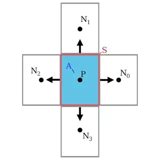
The Checkerboard Phenomenon
You might notice that although we only store the velocities at the cells's centers, we need the velocities at their faces. This can be approximated by linearly interpolating between the two cells the face is delimiting :
$$\vec v_s \approx \frac{\vec v_p + \vec v_n}{2}$$
When we expand the sum, this approximation has the notable effect of removing any reference to the center cell :
$$\vec \nabla \cdot \vec v_p = \frac{1}{A} \sum_{sides} L \hat n \cdot \vec v_s = \frac{1}{A} \left(L_x(1;0)\cdot\vec v_{s0x} + L_y(0;1)\cdot\vec v_{s1y} + L_x(-1;0)\cdot\vec v_{s2x} + L_y(0;-1)\cdot\vec v_{s3y}\right)$$
Where $s0$ is the right edge, $s1$ the top, $s2$ the left and $s3$ the bottom.
$$= \frac{1}{A} \left(L_x v_{s0x} + L_y v_{s1y} - L_x v_{s2x} - L_y v_{s3y}\right) = \frac{1}{A} \left(L_x \frac{ v_{px} + v_{n0x}}{2} + L_y \frac{ v_{py} + v_{n1y}}{2} - L_x \frac{ v_{px} + v_{n2x}}{2} - L_y \frac{ v_{py} + v_{n3y}}{2}\right) = \frac{1}{A} \left(L_x \frac{ v_{n0x}-v_{n2x}}{2} + L_y \frac{ v_{n1y}-v_{n3y}}{2}\right)$$
And since when clearing the divergence :
$$ \frac{1}{A} \sum_{sides} L \hat n \cdot \left(\vec v_s - \hat n\frac{A}{4L}D\right) = 0 $$
$$ \frac{1}{A} \sum_{sides} L \hat n \cdot \left(\frac{\vec v_p + \vec v_n}{2} - \hat n\frac{A}{4L}D\right) = 0 $$
$$ \frac{1}{A} \sum_{sides} L \hat n \cdot \left(\frac{\vec v_p}{2} + \frac{\vec v_n - \hat n\frac{2A}{4L}D}{2}\right) = 0 $$
And in a similar fashion, $\vec v_p$ cancels itself.
This means that the divergence is only dependent on and only affects immediate neighbours and thus the center cell doesn't actually interact with its neighbors, leading to two "independent" simulations taking place.
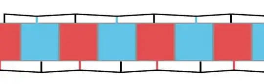
The two videos K.defaoite linked is part of a three-part series on the topic. The first part explains what I've just layed out and the two others give two different solutions to the problem. I decided to go with the staggered grid method, since it is the simplest and the fastest and is well suited for my usecase, although I highly reccommend watching both videos before making a decision, since both solutions have pros and cons.
Basically, the staggered grid method stores the velocities on the cell's sides instead of its centers, like so :

This means that when evaluating the divergence at the center of the cell, the side velocities are aleready available and when the divergence correction happens, it not only affects the neighboring cells's velocities, but also the center cell's.
This also explains the approach the author of this Github presentation took and why when I diverged from it, it didn't work.
Notes
- I have only shown the 2D version of this procedure, but it extends without modifications to other dimensions.
- All of this information is extrapolated from the previously mentioned Youtube channel.
- Although it might seem, from what I just showed, that only the parts of the velocities parallel to the normal (so only x components on left-right faces and y component on top-bottom faces) are needed to run the algorithm, nothing in the formulas necessitates it and I have found better stability when coupled to the advection step.
- I am aware that this question is long and may be full of errors. Please correct me in the comments or post your own answer, so I can correct my mistakes or point people towards a better source.


