There is no rule or theorem stating that sequential time-stepping is the only way to simulate evolution equations, but sequential time-stepping methods tend to be the easiest to implement and analyze. They also tend to be more efficient in terms of memory and and conditioning as the system at each time step is much smaller than solving for an entire spacetime field. Some problems do have an inherent sense of causality, such as hyperbolic equations, which impose restrictions on the type of time discretizations that yield consistent approximations.
However, there are methods that do full spacetime discretization that have been used. The two most prevalent methods to my knowledge are parallel-in-time algorithms (PITA) and space-time finite element methods.
Parallel-in-time algorithms such as Parareal work in the following way. To simulate the system $\dot{x} = f(x,t)$ on the interval $[0,T]$, you partition into coarse subintervals $[t_0,t_1]$, $[t_1,t_2]$, $\dots$, $[t_{n-1},t_n]$ where $t_0 = 0$ and $t_n=T$. You start with an intial guess for the solution value at each of these nodes, $x_0^0$, $x_1^0$, $\dots$, $x_{n-1}^0$ then simulate the following systems in parallel:
$$
\begin{aligned}
\dot{x}_0 &= f(x_0,t), \ x_0(t_0) = x_0^0, \ t\in[t_0,t_1] \\
\dot{x}_1 &= f(x_1,t), \ x_1(t_1) = x_1^0, \ t\in[t_1,t_2] \\
&\ \ \vdots \\
\dot{x}_{n-1} &= f(x_{n-1},t), \ x_{n-1}(0) = x_{n-1}^0, \ t\in[t_{n-1},t_n].
\end{aligned}
$$
This produces solutions over each subinterval computed in parallel, however the accuracy of these solutions is only as good as the initial guess provided and the solution may not be continuous. Enforcing continuity leads to the following conditions:
$$
\begin{aligned}
x_0(t_1) - x_1(t_1)&=0 \\
x_1(t_2) - x_2(t_2)&=0 \\
& \ \ \vdots \\
x_{n-2}(t_{n-1}) - x_{n-1}(t_{n-1})&=0.
\end{aligned}
$$
This can be written as a nonlinear system of the form $F(x)=0$, where $x$ is the vector of initial conditions for the subsystems and can be solved via Newton's method or various approximate Newton's methods for cheaper Jacobian calculations.
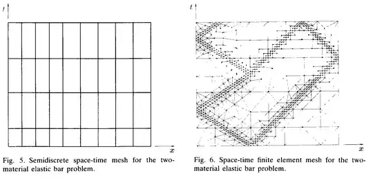
Space-time finite element methods work, as the name implies, by performing the finite element method over a mesh in both space and time as opposed to just space. This is advantageous for problems involving moving discontinuities, as the solution are truly discontinuous in both space and time, so traditional semidiscretizations can have trouble handling the discontinuity when time-stepping. An example is shown inthe below figure from Hughes 1990. On the left is a standard semidiscretization where space is discretized according to some scheme and time is simply partitioned into uniform subinvertvals for iteration. The figure on the right shows how a space-time mesh can be adapted to handle moving discontinuities in the solution, incrasing temporal fidelity and more accurately capturing sharp solution features while not overrefining the time step in regions where the solution is smooth.
Gander, Martin J.; Vandewalle, Stefan, Analysis of the parareal time-parallel time-integration method, SIAM J. Sci. Comput. 29, No. 2, 556-578 (2007). ZBL1141.65064.
Hulbert, Gregory M.; Hughes, Thomas J. R., Space-time finite element methods for second-order hyperbolic equations, Comput. Methods Appl. Mech. Eng. 84, No. 3, 327-348 (1990). ZBL0754.73085.
