14

Imagine a continuous one-dimensional line, which is duplicated exactly once. Duplication starts at random spacetime points. Once a point is duplicated, it starts a double duplication wave moving in either direction at constant speed $v$ (similar to a bi-directional zipper), as the following animation suggests

enter image description here

$I(x,t)$ is defined as the probability the position $x$, if not already duplicated at time $t$, initiates a double wave at time $t$.

Consider now a large number of lines and define $s(x,t)$ as the fraction of lines where position $x$ has not yet been duplicated ($I(x,t)$ is the same across all lines). From this definition, we may extract the probability distribution of duplication timing.

First, note that a position $x$ is not duplicated at time $t$ iff its duplication timing $t_D(x)$ is greater than $t$. Therefore the probability distribution $P(x,t)$ of the duplication timing at position $x$ is given by $$ P(x,t)=-\partial_t s(x,t) $$ as $s(x,t)=\text{Prob}(t_D(x)\geq t)$.

Question: In my modelling approach, I define the term $f(x)$, which is the rate of initiation at position $x$, constant in time, which should be related to $I(x,t)$ in some form. I am interested in determining the expected time of duplication at a given position $x$, defined as $\langle t_D(x)\rangle$ and inverting the problem: is it possible to write the initiation rate $f(x)$ in terms of $\langle t_D(x)\rangle$? $\langle t_D(x)\rangle$ has also been discussed here, from a different perspective.

My attempt: For infinite and continuous lines, this problem has been studied in the context of nucleation and replication. In particular, it was shown that, using light-cone coordinates, $$ s(x,t)=e^{-\int_{V_X[v]}dYI(Y)} $$ where $V_X[v]$ is the past light cone of the spacetime point $X=(x,t)$. This equation has the following elegant inverse, using the D'Alembert operator $\square=\frac{1}{v^2}\partial_t^2-\partial_x^2$, $$ I(x,t)=-\frac{v}{2}\square \log s(x,t) $$ On the other hand, given the probabilistic description provided before, we also have $$ \langle t_D(x)\rangle=\int_0^\infty tP(x,t)\,dt=-\int_0^\infty t\partial_ts(x,t)\,dt $$ However, from here, it is not clear how to rewrite this so that I have the rate $f(x)$ as a function of $\langle t_D(x)\rangle$. In particular, how are $I(x,t)$ and $f(x)$ related? The general steps could potentially be:

  1. Write $s(x,t)$ in terms of $\langle t_D(x)\rangle$.
  2. Use D'Alembert formula to write $I(x,t)$ in terms of $\langle t_D(x)\rangle$.
  3. Write $f(x)$ in terms of $I(x,t)$.
  4. What happens in the discrete space case, where duplication only starts at specific points $\{x_i\}$ (say integers in the real line, for simplicity)? For instance, what happens when $I(x,t)\equiv\sum_{y\in\mathbb{Z}}\delta(x-y)I(x,t)$?

Any ideas?

Other general ideas:

  • The inverse Laplace transform could prove useful to invert the previous equation, but not too sure how. Similarly, the Lambert W function could hold some useful information.
  • Initiation is a Poisson process where only the first event matters (there is no re-duplication), therefore can conditionality be relaxed and is there a direct relation between initiation rate $f(x)$ and probability $I(x,t)$ over time? In particular, due to the constant speed, waves do not overlap and the expected time should be the same nonetheless.
  • I am generally hoping for an elegant solution, but if not possible, where is the issue?
sam wolfe
  • 3,465

2 Answers2

3

I hope that I understood your modelling approach and terminology correctly. I will show how to get from $f(x)$ to $\mathbb{E}t_D(x)$ by analizing a general case first. I think going in the opposite direction is much harder because it involves "inverting a kernel".

Solution for Poisson point process

If we can assume that instances of "starts of duplication" (let's call them "pops") conform to Poisson point process, that is:

  • numbers of pops in disjoint regions of spacetime are independent random variables,
  • number of pops in a region of spacetime $A \subset \mathbb{R}\times\mathbb{R}^+ $ follows Poisson distribution with a parameter $\mu(A)$ where $\mu$ is some measure on $\mathbb{R}\times\mathbb{R}^+$,
  • $\mu(A)$ is finite for compact $A$ (technical assumption),

then we can arrive to a somewhat elegant solution.

Let $A_{x,t}$ denote the region in which the pop would need to occur in order to point $x$ get duplicated by the time $t$. In one dimensional case it is a triangle with vertices at: $$(x,t), (x-vt, 0), (x+vt, 0).$$

Let $N(A)$ be the (random) number of pops in region $A$, then $$t_D(x) > t \iff N(A_{x,t}) = 0$$

and $$\mathbb{P}(t_D(x) > t) = \mathbb{P}(N(A_{x,t}) = 0) = e^{-\mu(A_{x,t})}.$$

Using $\mathbb{E}X = \int_0^\infty \mathbb{P}(X>t)dt$, we get

$$\mathbb{E}t_D(x) = \int_0^\infty e^{-\mu(A_{x,t})} dt.$$

Solution for rate of initiation constant in time

For constant rate of initiation $f(x)$ we have $\mu(dxdt) = f(x)dxdt$. We can then calculate

$$\mu(A_{x,t}) = \int_{x-vt}^{x+vt}f(y)(t-|x-y|/v)dy $$

and plug that into the formula for $\mathbb{E}t_D(x)$.

For constant $f(x)=f$ we get $\mu(A_{x,t}) = f vt^2$ and

$$ \mathbb{E}t_D(x) = \int_0^\infty e^{-fvt^2} dt = \frac12\sqrt{\frac{\pi}{fv}} $$

mbartczak
  • 653
  • This is an interesting approach. However, I am still struggling to understand something. For example, if we take a constant initiation rate (in space-time), say $f(x)=f$, I would expect to get, in light-cone coordinates, $s(x,t)=1-e^{-\int_0^t \int_{x-vt}^{x+vt}f,dy,dt}=1-e^{-f vt^2} $ and thus $\mathbb{E}t_D(x)=\frac12\sqrt{\frac{\pi}{fv}}$, where naturally the $x$ dependence is non-existent here. However, I do not seem to get that from your deduction. Any ideas? – sam wolfe Feb 01 '24 at 12:00
  • Also, what do you mean by an exponential distribution "along dt"? If space is discrete, the time it takes for a site to pop follows an exponential, but I don't see the analogy in the continuous case. Interestingly, the $\frac12\sqrt{\frac{\pi}{fv}}$ estimate also arises in the discrete case, but the goal is to unify this framework. – sam wolfe Feb 01 '24 at 12:03
  • One last comment. I might be influenced by the discrete case, and where each discrete site pops with a rate $f(x)$, and some terminology might be wrong, but I wonder whether it is relatively possible to shift between continuous and discrete settings. In this paper (page 10, eq 5), they consider discrete "popping" by using delta functions, but it is not clear to me whether the explicit calculation of $\mathbb{E}t_d$ can be achieved. A bit of an overkill, but hopefully this sheds some light on the problem I am trying to solve. – sam wolfe Feb 01 '24 at 12:09
  • Oh, you are right! It is the time of the first pop that is "exponential along dt" when the intensity is constant, as it should be. It that case $\mu(dxdt) = f(x)dxdt$ and you calculation checks out :) I will edit the answer to fix this – mbartczak Feb 02 '24 at 19:37
  • The reasoning easily generalizes to discrete or even mixed settings and will work with all kinds of measures $\mu$. Let's say you want to model "pops" only occurring at integer points (with intensities $f_n$), you would then get $\mu(A_{x,t}) = \sum_n f_n \max(t-|x-n|/v, 0)$ – mbartczak Feb 02 '24 at 20:17
  • Thanks! I might have overused the variable $t$, but you get it. I think I understand where the "deeper" problem might lie. The data I have is on the discrete position-dependent mean time of duplication ($\mathbb{E}t_D(x_i)$). However, the d'Alembert formula is written in terms of $s(x,t)$. While $\mathbb{E}t_D(x_i)=-\int_0^\infty t \partial_ts(x,t),dt$, I am not sure I can invert this and apply the fitting to get $I(x,t)$ in terms of $\mathbb{E}t_D(x_i)$. If $I(x,t)=f$, it's easy to invert. Perhaps something with Laplace transforms or Lambert W functions could tell more. Is this issue clear? – sam wolfe Feb 02 '24 at 21:55
  • Also, I think the measure in the discrete case would be written in terms of Dirac delta functions, right? Are you able to write that specifically? See here. – sam wolfe Feb 02 '24 at 21:58
  • You could write $\mu(dxdt) = (\sum_{n}f_n\delta(dx-n))dt$ – mbartczak Feb 04 '24 at 12:31
  • If you're after analytical solution, one thing that might be helpful in solving the PDE is to apply Fourier transform wrt space dimension.

    If it's rather the case of fitting $f(x)$ to experimental data I would try simulating different initiation measures (eg. one atom, multiple atoms, gaussian, uniform over interval, triangle over interval, etc.) and analyze how they influence $\mathbb{E}t_D(x)$ to come up with some heuristics for the optimization problem "find $f(x)$ that best explains observed $\mathbb{E}t_D(x)$"

    – mbartczak Feb 04 '24 at 12:41
1

I provide some literature about modeling .

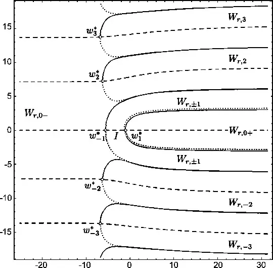
lambertW

See the reference 2. for the picture

Reference :

  1. https://arxiv.org/abs/0912.4554v5
  2. https://www.sciencedirect.com/science/article/pii/S0022247X17305218
  3. https://d-nb.info/993110037/34

For a physical interpretation see wave pendulum with same length and on the same line at $t=0$ .

Well it's not wave pendulum it's Newton's pendulum n

Remark : we can follow a very different way with Laplacian operator and Feynman-Kac formula see Solving a PDE with Feynman-Kac Formula

Barackouda
  • 3,879
  • 1
    Lambert W functions are exciting! Can you expand more on how to relate them to my problem? I initially thought of using an inverse Laplace transform, but that does not seem to lead anywhere. Any further ideas? – sam wolfe Feb 02 '24 at 21:48
  • @samwolfe The paper is a bit hard for me but this one is understandable and provide a lower bound https://userweb.ucs.louisiana.edu/~xxw6637/papers/ASY2014.pdf . It use the Grönwall lemma and use Lambert W – Barackouda Feb 03 '24 at 08:21