Does Radon-Nikodym derivative affect the Variance of a Random Variable?

Question

Edit 26 January 2022: The answer below elegantly shows that when the diffusion term of an Ito process is not constant in $\omega$, it is generally not true that Variance remains unaffected by the change of measure.

In the question below, however, the focus is on the case where the diffusion term of the stochastic process is constant. I would therefore appreciate any additional answers that would focus on the case with constant diffusion term. Additionally, it would be amazing to make a link between the continuous and the discrete case that are discussed below.

Original question:

Suppose $$X_t:=W^{\mathbb{P}}_t+\mu t$$ with $W^{\mathbb{P}}$ being the standard Wiener process under $\mathbb{P}$. We know that trivially, under $\mathbb{P}$, the PDF for $X_t$ would be:

$$f_{X_t}(h)=\frac{1}{\sqrt{t2\pi }}\exp\left(\frac{-(h-\mu t)^2}{2t}\right)$$

The Cameron-Martin-Girsanov theorem gives us the Radon-Nikodym derivative that will turn $X_t$ into a standard Wiener process under some new $\mathbb{Q}$, specifically:

$$\frac{d\mathbb{Q}}{d\mathbb{P}}=\exp\left(\frac{-2X_t\mu t+\mu^2t^2}{2t}\right)=\exp\left(-X_t\mu +0.5\mu^2t\right)=\exp\left(-W_t\mu -0.5\mu^2t\right)$$

Under $\mathbb{Q}$, the PDF for $X_t$ now becomes:

$$f_{X_t}(h)=\frac{1}{\sqrt{t2\pi }}\exp\left(\frac{-h^2}{2t}\right)$$

Bottom line: changing the measure has resulted in a different mean, but the variance has been preserved (it remains $t$ under both measures).

Question: I came up with a toy example to illustrate a change of measure on the following Binomial tree, but the change of measure seems to have produced a change in the variance. Was I wrong to assume that change of measure always preserves variance? Is there a proof that shows otherwise?

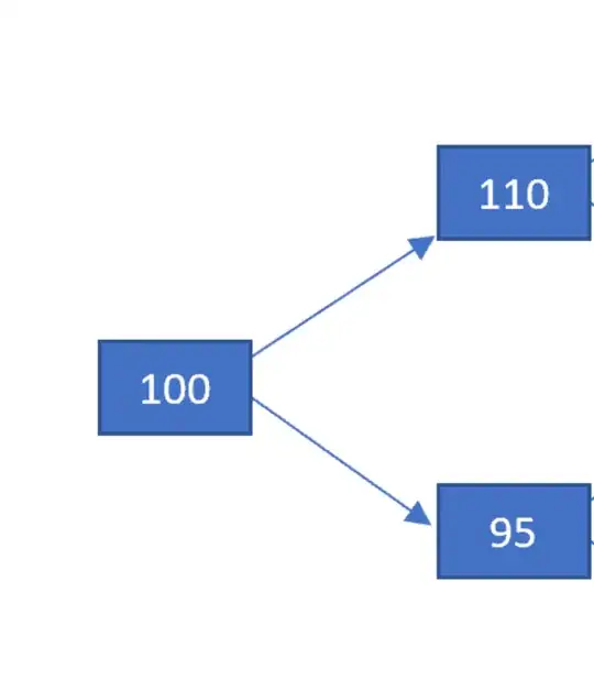
Toy example: $X_t$ is now a single-period variable, which can take the values {$110,95$} with equal probabilities of 0.5 under $\mathbb{P}$:

Under $\mathbb{P}$, we have: $$\mathbb{E}^{\mathbb{P}}[X_1]=0.5*110 + 0.5 * 95 = 102.5$$ (note that the "drift" is 2.5% per this single period, i.e. on "average", we move to 102.5 from the initial value of 100),

whilst we have $$Var^{\mathbb{P}}(X_1)=\mathbb{E}^{\mathbb{P}}[(X_1-102.5)^2]=0.5*7.5^2+0.5*7.5^2=56.25$$

Now we define $\frac{d\mathbb{Q}}{d\mathbb{P}}(\omega)=\frac{2}{3}$ when $X_1=110$ and $\frac{d\mathbb{Q}}{d\mathbb{P}}(\omega)=\frac{4}{3}$ when $X_1=95$: this results in the probability of $X_1$ being "up" changing from $0.5$ to $\frac{1}{3}$ whilst the probability of $X_1$ being "down" changes from $0.5$ to $\frac{2}{3}$. As a result, we now have:

$$\mathbb{E}^{\mathbb{Q}}[X_1]=\mathbb{E}^{\mathbb{P}}\left[X_1\frac{d\mathbb{Q}}{d\mathbb{P}}(\omega)\right]=\frac{1}{2}*\frac{2}{3}*110+\frac{1}{2}*\frac{4}{3}*95=100$$ (note that we have eliminated the "drift" via change of measure),

whilst we have

$$Var^{\mathbb{Q}}(X_1)=\mathbb{E}^{\mathbb{Q}}[(X_1-100)^2]=\frac{1}{3}*10^2+\frac{2}{3}*5^2=50$$

(note that unfortunately, we have also changed the variance)

What worries me further is that this paper shows that the multiplicative Binomial tree model converges to the well-known Geometric-Brownian-Motion (GBM) model when we take the limit in the Binomial tree of time-step converging to zero: and the C-M-G theorem is regularly applied to the GBM model to change measure such that the drift term changes, whilst the Variance remains the same: I therefore assumed that taking the Binomial tree as a toy example would be safe to achieve a similar result (i.e. changing the measure to eliminate "drift", whilst preserving the variance of $X_t$).

Thank you for any hints and tips.

Answer 1

Not an answer (but too long for a comment). For definitions, conventions and notations, see my posts [1, 2].

Let the price process $S_t$ be an Itô process: $$S_t=S_0+\int_0^tb_s\,\mathrm ds+\int_0^t \sigma_s\,\mathrm dW_s.$$ Assume for illustrative purposes first that $b_s(\omega)=\mu\in\mathbb R$ for all $s\in[0,T]$ and $\omega\in\Omega$.

Then $$\mathsf V^{\mathsf P}(S_t)=\mathsf V^P\left(\int_0^t\sigma_s\,\mathrm dW_s\right).$$

In the setting of the equivalent martingale measure, as derived in [1, 2], we have $$S_t=S_0+\int_0^t \sigma_s\,\mathrm dW_s^{\mathsf Q}.$$

So $$\mathsf V^{\mathsf Q}(S_t)=\mathsf V^{\mathsf Q}\left(\int_0^t\sigma_s\,\mathrm dW_s^{\mathsf Q}\right).$$

As is assumed in [1, 2], the process $\sigma$ must be progressively measurable with $\mathsf E\left(\int_0^T \sigma_s^2\,\mathrm ds\right)<\infty$. In that case, $\int_0^t\sigma_s\,\mathrm dW_s$ is a $\mathsf P$-martingale and $\int_0^t\sigma_s\,\mathrm dW_s^{\mathsf Q}$ is a $\mathsf Q$-martingale [3; Satz 25.17 (iii)].

By [3; Korollar 25.19 & Satz 21.70(ii)] we thus have that $\left(\int_0^t\sigma_s\,\mathrm dW_s^{\mathsf Q}\right)^2-\int_0^t \sigma_s^2\,\mathrm ds$ and $\left(\int_0^t\sigma_s\,\mathrm dW_s\right)^2-\int_0^t \sigma_s^2\,\mathrm ds$ are $\mathsf Q$- and $\mathsf P$-martingales, respectively, both null at $t=0$, so that $$\mathsf V^{\mathsf Q}\left(\int_0^t\sigma_s\,\mathrm dW_s^{\mathsf Q}\right)=\mathsf E^{\mathsf Q}\left(\int_0^t \sigma_s^2\,\mathrm ds\right)$$ and $$\mathsf V^{\mathsf P}\left(\int_0^t\sigma_s\,\mathrm dW_s^{\mathsf P}\right)=\mathsf E^{\mathsf P}\left(\int_0^t \sigma_s^2\,\mathrm ds\right).$$

In particular, it is in general not true that $$\mathsf V^{\mathsf P}(S_t)=\mathsf V^{\mathsf Q}(S_t),$$ even if we assume constant drift.

---

This doesn't answer your question though because if $\sigma$ is constant in $\omega$ then we do have $\mathsf V^{\mathsf P}(S_t)=\mathsf V^{\mathsf Q}(S_t)$. And it seems at first sight that in the binomial tree model written as some sort of discrete Itô process (which I do not know how to do right now), $\sigma$ would be constant.

---

Literature

[1] Maximilian Janisch, What does the VIX measure?, https://quant.stackexchange.com/a/69494/51954.
[2] Maximilian Janisch, Why does the diffusion term remain the same when we change pricing measure?, https://quant.stackexchange.com/a/69623/51954.
[3] Achim Klenke, Wahrscheinlichkeitstheorie. 3. Auflage. Springer-Verlag Berlin/Heidelberg (2013).