Biggest circle under a polynomial curve

Question

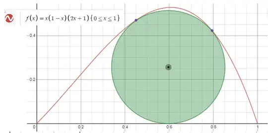
What is the biggest circle that is contained in the region bounded by the graph of the polynomial $f(x) = x(1-x)(2x+1)$ and the x-axis interval $[0, 1]$?

(Here's the thing in Desmos)

---

Here's what I have tried

Let's denote the center of the circle by $(c_x, c_y)$ and the points of tangency by $(x_k, y_k)$, $k=1,2$. From distance to the x-axis, we know that the radius of the circle is then $c_y$. We can express the tangency by the dot product of the vectors $(x_k-c_x, y_k-c_y)$ and $(1, f'(x_k))$ being zero. So we get the group of equations (all for $k=1,2$)

$$\begin{cases} (x_k-c_x)^2 + (y_k-c_y)^2 &=& c_y^2 \\ x_k-c_x + (y_k-c_y)f'(x_k) &=& 0 \\ f(x_k) &=& y_k \end{cases} $$

Then I tried to solve this group by using Gröbner basis and elimination ideals. I wrote this SageMath code:

f(x) = x*(1-x)(2*x+1)
fd = f.derivative()
R.<x1, y1, x2, y2, cx, cy> = PolynomialRing(QQ, order='lex')
polys1 = [(cx-xk)2+(cy-yk)2 - cy*2 for (xk, yk) in [(x1,y1), (x2, y2)]]
polys2 = [(xk-cx)+(yk-cy)fd(xk)  for (xk, yk) in [(x1,y1), (x2, y2)]]
polys3 = [f(xk)-yk for (xk, yk) in [(x1,y1), (x2, y2)]]
I = R.ideal(polys1+polys2+polys3)
gb = I.groebner_basis()
for poly in gb:
    print (poly)
print (I.dimension())

It gave me a long list of polynomials, the last one being

$$c_x^6 - 2c_x^4c_y^2 + \frac{5}{4}c_x^4c_y + \frac{1}{64}c_x^4 + c_x^2c_y^4 + \frac{3}{4}c_x^2c_y^3 + \frac{3}{16}c_x^2c_y^2 + \frac{1}{64}c_x^2c_y$$

and said the dimension is $1$. I now realize the reason we don't get dimension $0$ has probably to do with the fact that the points $(x_1, y_1)$ and $(x_2, y_2)$ could be the same point(?) So for a solution, the point $(c_x, c_y)$ should be a zero of that polynomial? But is even that correct, since the points could be collapsed and the other side go over the curve??

How to solve this even numerically? I tried with Sage by minimizing the square sum of all those polynomials that should be zero. I also tried adding constraints for the variables to be near the solution that can be seen from the picture but that didn't work either.

Answer 1

We have

$$ \cases{ y = x(1-x)(2x+1)\\ (x-x_0)^2+(y-y_0)^2=y_0^2 } $$

substituting the first into the second we have

$$ p(x)=(x-x_0)^2+(x(1-x)(2x+1)-y_0)^2-y_0^2 = 0 $$

This polynomial at tangency should have the following structure

$$ p(x) = c(x-x_1)^2(x-x_2)^2((x-a)^2+b^2)\ \ \ \ (\text{Why?}) $$

now comparing coefficients we have

$$ 0=\eta = \left\{ \begin{array}{l} x_0^2-c x_1^2 x_2^2 \left(a^2+b^2\right) \\ 2 c x_1 x_2 \left(x_2 \left(a^2+b^2\right)+x_1 \left(a^2-a x_2+b^2\right)\right)-2 x_0-2 y_0 \\ 2 -c x_1^2 \left(a^2-4 a x_2+b^2+x_2^2\right)-4 c x_2 x_1 \left(a^2-a x_2+b^2\right)-c x_2^2 \left(a^2+b^2\right)-2 y_0 \\ 2 \left(c x_1 \left(a^2-4 a x_2+b^2+x_2^2\right)+c x_2 \left(a^2-a x_2+b^2\right)+c x_1^2 \left(x_2-a\right)+2 y_0+1\right) \\ c \left(a^2+b^2\right)+c \left(4 x_1 \left(x_2-a\right)+x_2 \left(x_2-4 a\right)+x_1^2\right)+3 \\ 2 c \left(x_1+x_2\right)-2 (a c+2) \\ 4-c \\ \end{array} \right. $$

and we finish by solving this nonlinear system for $x_0,y_0,x_1,x_2,a,b,c$ using a minimization procedure such as

$$ \min_{x_0,y_0,x_1,x_2,a,b,c} \eta\cdot\eta\ \ \ \text{s. t.}\ \ \ \{x_0 > 0,y_0 >0, x_1 > 0, x_2 > 0\} $$

Follows a MATHEMATICA script which materializes those computations

Clear[g1, g2]
g1[x_, y_] := y - x (1 - x) (2 x + 1)
g2[x_, y_] := (x - x0)^2 + (y - y0)^2 - y0^2
dif = g2[x, x (1 - x) (2 x + 1)] - c (x - x1)^2 (x - x2)^2 ((x + a)^2 + b^2)
eta = CoefficientList[dif, x]
sol = NMinimize[{eta.eta, x0 > 0, y0 > 0,x1 > 0, x2 > 0}, {x0, y0, x1, x2, a, b, c }]
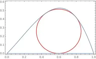
g2x = g2[x, y] /. sol[[2]]
gr1 = ContourPlot[g2x == 0, {x, 0, 1}, {y, 0, 0.6}, ContourStyle -> Red];
gr2 = ContourPlot[g1[x, y] == 0, {x, 0, 1}, {y, 0, 0.6}];
gr3 = Plot[0, {x, 0, 1}]
Show[gr1, gr2, gr3, AxesOrigin -> {0, 0}, AspectRatio -> 0.6]

Answer 2

I now managed to solve it at least numerically with Sage. I first find the closest point on the curve to a given point $(c_x, c_y)$. This can be done by finding the minimum of

$$(x-c_x)^2 + (f(x)-c_y)^2$$

by finding roots of its derivative (equivalent to the "tangency equation")

$$12x^5-10x^4-6x^3+(3+6c_y)x^2+(2-2c_y)x-c_x-c_y.$$

This allows to write the constraint for the radius.

Here's another Desmos link to test it out.

Take the radius $r$ to be another variable, having just $c_x$ and $c_y$ didn't work for some reason (the radius constraint was violated in the answer).

f(x) = -2.0*x**3 + x**2 + x
fd = f.derivative()
def find_closest_on_curve(cx, cy):
    bestP = None
    bestD = None
    #for r in (x-cx+(f-cy)fd).roots(ring=CDF): #gives bug!!?!?!?
    for r in numpy.roots([12, -10, -6, 3+6cy, 2-2cy, -cx-cy]):
        #print (r)
        imag = r.imag
        real = r.real
        if abs(imag)<0.000001 and 0<=real and real<=1:
            xVal = real
            yVal = f(xVal)
            d = (xVal-cx)2+(yVal-cy)*2
            if bestP==None or d<bestD:
                bestP = (xVal, yVal)
                bestD = d
    return bestP
def radius_constraint(p):
    cx, cy, r = p
    closeP = find_closest_on_curve(cx, cy)
    if not closeP: return -1
    d = (cx-closeP[0])2 + (cy-closeP[1])2
    return min(d, cy2)-r2
constraints = ([
    lambda p: p[0]-0.3,
    lambda p: 0.7-p[0],
    lambda p: p[1]-0.1,
    lambda p: 0.4-p[1],
    lambda p: p[2],
    radius_constraint
])
startP = (0.6, 0.2, 0.1)
#print (radius_constraint(startP))
sol = minimize_constrained(lambda p: -p[2], constraints, startP)
print (sol)
#print (radius_constraint(sol))
g = Graphics()
g += plot(f, 0, 1)
nn=20
for (cx, cy, r) in [sol]:
    solP = find_closest_on_curve(cx, cy)
    #print (solP)
    if not solP: continue
    x1,y1 = solP
    g += points([(cx, cy), (x1, y1)])
    g += line([(cx, cy), (x1, y1)])
    g += circle((cx, cy), r, color="green")
g.show(aspect_ratio=1)

It gives the solution $(c_x, c_y, r) = (0.5965, 0.2577, 0.2577)$

Answer 3

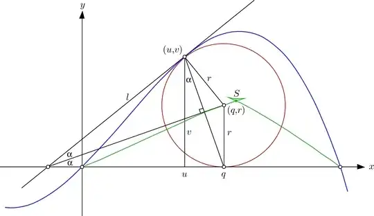
When $(u,v)$ is a point on your curve $\gamma: \>y=f(x)$ then we have $$v=f(u)=u+u^2-2u^3,\qquad m:=f'(u)=1+2u+6u^2\ .$$ Given $u$, $v$, $m$ there is exactly one circle touching $\gamma$ at $(u,v)$ as well as the $x$-axis at some $q$. This circle has a center $(q,r)$ and a radius $r$. In order to compute $q$ and $r$ we introduce the following quantities (see the figure): $$\tan(2\alpha)=m,\quad l={v\over\sin(2\alpha)}\ .$$ Then $$\eqalign{q(u)&=u+v\tan\alpha=u+v\>{\sqrt{1+m^2}-1\over m},\cr r(u)&=l\tan\alpha=v\>{1+m^2-\sqrt{1+m^2}\over m^2}\ .\cr}\tag{1}$$ This leads to the green curve $$u\mapsto\bigl(q(u),r(u)\bigr)\qquad(0\leq u\leq1)$$ in the figure. Each point of this curve is the center of a circle that touches $\gamma$ and the $x$-axis. This curve has a point $S$ of selfintersection, coming from two values $u_1\approx0.4507$, $u_2\approx0.7940$. The circle centered at this point touches $\gamma$ in two points $(u_i,v_i)\in\gamma$ as well as the $x$-axis, and it seems that this circle is the solution to your problem. The point $S\approx(0.5962,0.2578)$ can be found numerically with arbitrary precision, using the equations coming from $(1)$.