Error in Crank-Nicolson scheme for diffusion equation

Question

I'm solving the diffusion equation

$$\frac{\partial u}{\partial t}=D\frac{\partial^2u}{\partial^2x}$$

subject to the BCs $\partial_xu(x=0)=0$ and $u(x)=1$, using the Crank Nicolson scheme. For the middle points I'm using

$$\frac{u_i^{n+1}-u_i^n}{\Delta t}=\frac{1}{2}D\frac{u_{i+1}^n-2u_i^n+u_{i+1}^n}{\Delta x^2}+\frac{1}{2}D\frac{u_{i+1}^{n+1}-2u_i^{n+1}+u_{i+1}^{n+1}}{\Delta x^2},$$

whereas in the left point, I make use of the fact that $\frac{u_1-u_{-1}}{2\Delta x}=0\implies u_1=u_{-1}$ and thus write

$$\frac{u_0^{n+1}-u_0^n}{\Delta t}=\frac{1}{2}D\frac{2(u_{1}^n-u_0^n)}{\Delta x^2}+\frac{1}{2}D\frac{2(u_{1}^{n+1}-u_0^{n+1})}{\Delta x^2}.$$

When an initial condition $u(0,x)$ is given, I can also find the analytical solution of this equation and thus compare the simulation with theory.

I am evaluating the absolute error $||\mathbf{T_{simul}}-\mathbf{T_{anal}}||$ at each time $t$.

When $t\rightarrow\infty$, the solution goes to zero with machine precision, which makes sense.

Now let's say I pick up a time $t$, when heat is still diffusing, and evaluate the error, and then I make the same thing for a different time-step $\Delta t$.

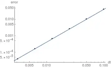
The resultant log-plot of the error with $\Delta t$ is the following:

The points fit very well with a linear function, but because this is a second-order scheme in $\Delta t$, I was expecting that the error would go with $(\Delta t)^2$ and not $\Delta t$!

EDIT: As suggested in the comments, the log-log plot is:

(This fit is made to a function of the type $a+b(\Delta t)^2$. I have been told however that the fit should not contain the constant term.)

---

FINAL EDIT:

With the help of @LutzL I have realized I was making one mistake in my code, namely I was comparing theory and simulation at times separated precisely by $\Delta t$.

Besides that, I have found the following very interesting results:

1) If I use as initial condition

$$u(x,0)=1.0+\cos\left(\frac{\pi}{2}x\right),$$

which gives the exact solution (with $D=1$)

$$u(x,t)=1.0+e^{-\pi^2t/4}\cos\left(\frac{\pi}{2}x\right)$$

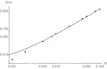
in the domain $x\in[0,1]$, I get that the error indeed goes with $(\Delta t)^2$:

The blue line gives the fit $4.106(\Delta t)^2$

2) Now if I use as initial condition

$$u(x,0)=1.0+\cos\left(\frac{x}{2}\right),$$

which gives the exact solution (with $D=1$)

$$u(x,t)=1.0+e^{-t/4}\cos\left(\frac{x}{2}\right)$$

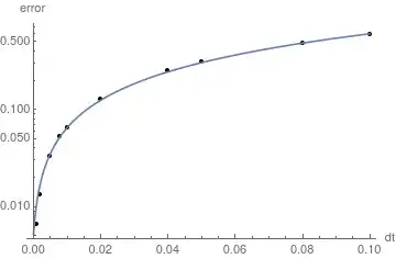
in the domain $x\in[0,\pi]$, I get the following trend for the error:

where the blue line is the fit $0.00135462 + 0.00283811x + 0.0239431x^2$

It is strange that the simple change of variable $\pi x\rightarrow x$ makes this behaviour. Note also that in both cases 1) and 2) I have kept $\Delta r=0.001$ fixed.

Answer 1

If you did everything right the matrix should have been constructed as follows or similar. The dynamic is in the inner points. Thus the approximation of $F$ gets the vector $(u_1,...,u_N)$ as input. The right boundary condition gives $u_{N+1}=1$. To reconstruct $u_0$ use the forward differentiation formula $$u_x(x=0)=\frac{3u_0-4u_1+u_2}{Δx}+O(Δx^2)$$ so that $u_0=\frac13(4u_1-u_2)$. With that the second derivative at the first position is approximated by $$ (u_{xx})_1=\frac{\frac13(4u_1-u_2)-2u_1+u_2}{Δx^2}=\frac{-2u_1+2u_2}{3Δx^2} $$ This gives the matrix for $F(u)=Au+b$ as $$ A=D\frac{Δt}{Δx^2} \pmatrix{ -\frac23&\frac23&0&\dots\\ 1&-2&1&0&\dots\\ &\ddots&\ddots&\ddots\\ \dots&0&1&-2&1\\ &\dots&0&1&-2 }, ~~~ b=D\frac{Δt}{Δx^2}\pmatrix{0\\0\\\vdots\\0\\1}. $$

Building a test case

Continuous problem with exact solution

$u_t=u_{xx}$, that is, $D=1$, with $u_x(0,t)=0$, $u(\pi,t)=1$ over $t\in[0,1]$.

Separation of variables tells us that terms $e^{-\omega^2t}\cos(\omega t)$ are simple functions that satisfy homogeneous condition automatically, using a constant for the shift gives as solution example $$u(x,t)=1+a_1e^{-t/4}\cos(x/2)+a_3e^{-9t/4}\cos(3x/2).$$

Code snippets (python, using scipy.sparse)

• the test solution

  a1, a3 = 2,1;
  def u_exact(x,t): return 1+a1*np.exp(-0.25*t)*np.cos(0.5*x)+a3*np.exp(-2.25*t)*np.cos(1.5*x)
  

• construction of the system matrices

  I = sparse.eye( M, format="csc" )
  A = sparse.diags([1, -2, 1], [-1, 0, 1], shape=(M, M), format="csc");
  A[0,0]=-2.; A[0,1]=2.;
  b = np.zeros(M); b[-1]=1
  

• the time iteration

  x = np.linspace(0,np.pi,M+1); dx = x[1]-x[0];
  u1 = u_exact(x,0)[:-1];
  t = np.linspace(0,T,N+1); dt = t[1]-t[0];
  p = dt/dx**2;
  for n in range(N):
      u1 = sparse.linalg.spsolve(I-0.5*p*A, (I+0.5*p*A).dot(u1)+p*b)
  

Numerical results

Using the left side BC treatment like in the question, I get the following table of results. Horizontally $M$ varies over the size of the space subdivision, while vertically $N$ gives the number of time steps.

In each cell the upper value is the error against a run with half the time step, which is an estimate of the error against exact time integration. The lower value is the error against the exact solution. The errors displayed is an approximation of the $L^2$ norm, that is, the Euclidean norm divided by $\sqrt M$. One can see that where $\frac{Δt}{Δx^2}$ gets small, the error against the exact solution becomes constant.

\begin{array}{|c|l|l|l|l|l|}\hline & ~M=10& ~M=50& ~M=200& ~M=1000& ~M=5000 \\ \hline N=10 & \begin{split} 5.5166e-04 \\ 2.6801e-03 \end{split} & \begin{split} 5.3780e-04 \\ 5.9059e-04 \end{split} & \begin{split} 5.3395e-04 \\ 7.0361e-04 \end{split} & \begin{split} 5.3286e-04 \\ 7.0966e-04 \end{split} & \begin{split} 5.3264e-04 \\ 7.0967e-04 \end{split} \\ \hline N=20 & \begin{split} 1.3755e-04 \\ 3.2229e-03 \end{split} & \begin{split} 1.3409e-04 \\ 5.6237e-05 \end{split} & \begin{split} 1.3313e-04 \\ 1.6967e-04 \end{split} & \begin{split} 1.3286e-04 \\ 1.7680e-04 \end{split} & \begin{split} 1.3280e-04 \\ 1.7703e-04 \end{split} \\ \hline N=40 & \begin{split} 3.4365e-05 \\ 3.3587e-03 \end{split} & \begin{split} 3.3500e-05 \\ 8.4139e-05 \end{split} & \begin{split} 3.3260e-05 \\ 3.6555e-05 \end{split} & \begin{split} 3.3193e-05 \\ 4.3943e-05 \end{split} & \begin{split} 3.3179e-05 \\ 4.4224e-05 \end{split} \\ \hline N=80 & \begin{split} 8.5898e-06 \\ 3.3927e-03 \end{split} & \begin{split} 8.3736e-06 \\ 1.1693e-04 \end{split} & \begin{split} 8.3137e-06 \\ 3.5075e-06 \end{split} & \begin{split} 8.2968e-06 \\ 1.0751e-05 \end{split} & \begin{split} 8.2933e-06 \\ 1.1045e-05 \end{split} \\ \hline N=160 & \begin{split} 2.1474e-06 \\ 3.4011e-03 \end{split} & \begin{split} 2.0933e-06 \\ 1.2518e-04 \end{split} & \begin{split} 2.0783e-06 \\ 5.1960e-06 \end{split} & \begin{split} 2.0741e-06 \\ 2.4544e-06 \end{split} & \begin{split} 2.0733e-06 \\ 2.7519e-06 \end{split} \\ \hline N=320 & \begin{split} 5.3683e-07 \\ 3.4033e-03 \end{split} & \begin{split} 5.2333e-07 \\ 1.2725e-04 \end{split} & \begin{split} 5.1958e-07 \\ 7.2298e-06 \end{split} & \begin{split} 5.1852e-07 \\ 3.8307e-07 \end{split} & \begin{split} 5.1832e-07 \\ 6.7867e-07 \end{split} \\ \hline \end{array}

Speculation

Without knowing details of the code used, there are two typical places that come to mind that might introduce a first order error:

• a wrong coefficient somewhere, reducing the method to first order. This is unlikely as the matrix and function in general has a simple structure. If there were an error one would expect more grave consequences.

• an error in the implementation of the time iteration. Such as

  • iterating N times but setting dt=T/(N-1), or
  • having T and dt as input and iterating while t<T without caring that the final t can be anywhere between T and T+dt.

  Such error results in a time difference between exact and numerical solution of order O(dt) which gives a difference in the function values of also O(dt).

Answer 2

The standard approach is to look to the log-log graph, interpolate a line and then to look at its slope. For polynomial order methods you get always a line in the log-log graph - not a curve! On the horizontal axis number of point per unit interval $N=\frac{1}{\triangle t}$ is usually used, in this way you get a decaying line. If the line slope is 1 then the method has order 1, if 2 then the method has order 2. It seems that you get the order close to 1 only, the question is why. If so, I would suggest to compare your Crank-Nicolson scheme with the multistep method of order 2 in time: \begin{equation} f'(0)=\frac{3f(0)-4f(-\triangle t)+f(-2\triangle t)}{\triangle t}+O(\triangle t^3) \end{equation} Another option could be the Runge-Kutta method of order 2 in time. You should get slope 2. Also, it is necessary to look to sufficiently small $\triangle t$, for higher values of $\triangle t$ the order could be worse than theoretically expected. Also, I suggest to use such a series of time steps, where each new trial is an exactly one half of the previous one: $\triangle t, \triangle t/2, \triangle t/4, \triangle t/8, \dots$ and to evaluate the error at some fixed time step, for example at $t=\triangle t$.