Find the critical region and the power when $H_0$ is false.

Question

In a sample $N(0, \sigma ^2)$ we have two hypothesis. $H_0: \sigma ^2 =16$ and $H_1: \sigma ^2 =4$

(a )For a sample of size n, find the form of the best critical region.

(b) If n = 10 and $\alpha = 0.10$, find the critical region and the power when $H_0$ is false.

(c) Whith the next sample: 0.05, 1.58, 1.41, -0.01, -0.40, -1.39, -1.78, 1.03, 1.27, 0.23; ¿Which hypothesis should be accepted?

a) I use the Neyman-Pearson Lemma:

$$\frac{L(16)}{L(4)} =\frac{\prod_{i=0}^n 1/\sqrt{32\pi} e^{\frac{-x_i^2}{32}}}{\prod_{i=0}^n 1/\sqrt{8\pi } e^{\frac{-x_i^2}{8}}} \le K$$

$$\iff \sum_{i=0}^n{X_i^2 \le c}$$

then $\gamma: $ Reject $H_0$ if $ \sum_{i=0}^n{X_i^2 \le c}$

thus the critical region is $C^*=\{(X_1,...,X_n) | \sum_{i=0}^n {X_i^2} \le c \}$

b)I think I should find the value of c using $P($Reject $ H_0 | H_a)$ and $\pi_\gamma (4) $ Is this correct?

In this case: $P($Reject $ H_0 | H_a) =P(\sum_{i=0}^n {X_i^2} \le c | \sigma^2=4)$ . Since $X_i^2=4(\frac{X_i}{2})^2 \sim$ Gamma$(1/2, 8)$ then $\sum_{i=0}^n {X_i^2} \sim$ Gamma $(5,8)$. If $\alpha=.1 $, c is the value of the quantile .1

c) $P($Reject $ H_0 | H_0) =P(\sum_{i=0}^n {X_i^2} \le c | \sigma^2=16)$ using the same argument in b) I get: $\sum_{i=0}^n {X_i^2} \sim$ Gamma $(5,32)$ and c=77.84, using the values $\sum_{i=0}^n {X_i^2}=12.47$ then $H_0 $ is rejected

Answer 1

You seem to be mainly on the right track with this problem. However, there are some mistakes in your Answer. My approach here follows traditional patterns of inference for the population variance of normal data when the population mean is known. (Perhaps see this Q & A.)

Suppose $X_1, \dots, X_n$ is a random sample from $\mathsf{Norm}(\mu, \sigma),$ with known $\mu$ and unknown $\sigma.$ Then the estimator $$V = \hat{\sigma^2} = \frac 1n\sum_{i=1}^n (S_i - \mu)^2$$ of $\sigma^2$ has $\frac{nV}{\sigma^2} \sim \mathsf{Chisq}(\nu = n).$ In your problem we know $\mu = 0.$

We can test $H_0: \sigma=^2 = 16$ vs. $H_a: \sigma^2 = 4$ using the statistic $V = \sum_{i=1}^10.$ As you say, we will reject for small values of $V.$

If $n = 10,$ the null distribution of $V$ has $\frac{10V}{16} \sim \mathsf{Chisq}(10),$ for which the lower decile is 4.865, as computed in R.

qchisq(.1, 10)
[1] 4.865182

Thus, the critical value at level $\alpha=0.1$ of the test in terms of $V$ is $(16/10)4.865 = 7.7843,$ This makes sense intuitively because we expect $V \approx 10$ when $H_0$ is true and $V \approx 4$ when $H_a$ is true, so that 7.7843 seems a reasonable value to separate the two contemplated values of $\sigma^2.$

[Note: The gamma distribution of $V$ under $H_0,$ can be expressed as $V \sim \mathsf{Gamma}(\text{shape}=5, \text{rate}=1/3.2).$ We can get the same critical value as above from this distribution.]

qgamma(.1, 5, 1/3.2)
[1] 7.784291

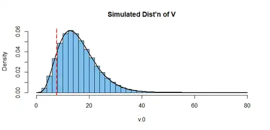
The histogram below is based on a simulation in R with a million samples of size ten from the null distribution. Except for simulating the power, I leave the details of the power computation to you.

v.0 = replicate(10^6, (1/10)*sum(rnorm(10, 0, 4)^2))
mean(v.0 < 7.7843)
[1] 0.100034           # significance level

hist(v.0, prob=T, br=30,  col="skyblue2",
     main="Simulated Dist'n of V")
  curve(dgamma(x, 5, 1/3.2), add=T, lwd=2)
  abline(v = 7.7843, col="red", lty="dashed", lwd=2)


set.seed(2019)
v.a = replicate(10^6, (1/10)*sum(rnorm(10, 0, 2)^2))
mean(v.a < 7.7843)
[1] 0.965331           # power against alt