Chi Square Contingency Table - Formula Derivation

Question

A chi-square distribution is constructed from normal random variables $X_{i=1, \dots ,n}$, each with normal distribution and mean $\mu$ and variance $\sigma^2$. Transforming to standard normal and squaring, i.e.:

$$\frac{(X_i - \bar{X})^2}{\operatorname{Var}(X_i)}\sim N(0,1)^2$$

Then add these over all your $n$ random variables, then you get $\chi^2_{n-1}$ - a chi-square with $n-1$ degrees of freedom.

For contingency tables, suppose there are $k$ categories of observations $O_i, i = 1, \ldots , k,$ each with probability $p_i$. The statistic we’re proposing, assuming $O_i \sim \operatorname{Normal}$, is:

$$\frac{(O_i-np_i)^2}{\operatorname{Var}(O_i)} \sim N(0,1)^2$$

The variance of each observation is $np_i(1-p_i)$

For contingency tables, a test to see if the underlying mean is the same across categories, the standard equation taught for calculating the Chi-Square statistic is:

$$\sum_{i=1}^k\frac{(O_i-np_i)^2}{np_i} \sim \chi^2_{n-1}$$

So, where in the equation for assessing contingency tables does the term $(1-p_i)$ disappear to?

Answer 1

Let the $n$-dimensional $\mathbf{X}$ be Multinomial$(N,\mathbf{p})$ distributed, where $\mathbf{p}$ is composed of $p_0, p_1, \dots, p_{n-1}$ and $N$ is the total count of the contingency table. Since the sum of components of $\mathbf{X}$ is always $N$, effectively there are only $n-1$ free variables.

So we may drop the first component by letting $$\begin{align}\mathbf{Y}&=(X_1, X_2, \dots, X_{n-1})^T,\text{ and }\\\mathbf{q}&=(p_1, p_2, \dots, p_{n-1})^T.\end{align}$$ It follows that the mean and variance of $\mathbf{Y}$ are $$\mathbf{\mu}:=\mathbb{E}(\mathbf{Y})=N\mathbf{q},\\ \mathbf{\Sigma}:=\mathbb{V}\mathrm{ar}(\mathbf{Y})=N\left[\operatorname{diag}(\mathbf{q})-\mathbf{qq}^T\right]. $$ For sufficiently large $N$, central limit theorem allows us to approximate the distribution of $\mathbf{Y}$ by multivariate normal distribution with the above mean and variance, and $$ (\mathbf{Y}-\mathbf{\mu})^T\mathbf{\Sigma}^{-1}(\mathbf{Y}-\mathbf{\mu})\stackrel{D}{\longrightarrow} \chi^2_{n-1}. $$ We will show that the LHS quadratic form is exactly the Pearson's $\chi^2$ statistic in this multinomial model.

By using Sherman-Morrison inversion formula (or Woodbury inversion), $$ \mathbf{\Sigma}^{-1} =\frac1N\operatorname{diag}\left(1/\mathbf{q}\right) + \frac1{Np_0} \mathbf{11}^T, $$where $\operatorname{diag}\left(1/\mathbf{q}\right)$ refers to a diagonal matrix with $1/q_i$ as the $i$th diagonal element. Now, $$\begin{align} &(\mathbf{Y}-\mathbf{\mu})^T\mathbf{\Sigma}^{-1}(\mathbf{Y}-\mathbf{\mu}) \\ =&\frac1N(\mathbf{Y}-N\mathbf{q})^T \operatorname{diag}\left(1/\mathbf{q}\right) (\mathbf{Y}-N\mathbf{q}) +\frac1{Np_0}(\mathbf{Y}-N\mathbf{q})^T \mathbf{11}^T (\mathbf{Y}-N\mathbf{q})\\ =&\frac1N\sum_{k=1}^{n-1} \frac{\left(Y_k -N q_k\right)^2}{q_k} + \frac1{Np_0}\left(\sum_{k=1}^{n-1}Y_i -N \sum_{k=1}^{n-1}q_k\right)^2. \end{align} $$ But because $\sum_{k=1}^{n-1}Y_i=N-X_0$ and $\sum_{k=1}^{n-1}q_k=1-p_0$, the second term above is simply $$\frac{ \left(-X_0 +Np_0\right)^2}{Np_0}, $$which can be combined to with the first term, resulting in $$ \chi^2 = \sum_{k=0}^{n-1} \frac{\left(X_k -N p_k\right)^2}{Np_k}, $$with summation over all $n$ categories (including the first). This finished the derivation.

PS: Note that nowhere in the derivation did we assume the cell counts being Poisson distributed. Our starting model is a Multinomial distribution. Although conditioning on the sum of independent Poissons will result in Multinomial distribution, most applied situations where $\chi^2$ test is used typically do not assume an underlying Poisson model.

Answer 2

One experiment. Illustration in terms of rolling a fair die. Suppose I use R statistical software to roll a fair die $n=600$ times, observing counts $X = (104, 96, 96, 104, 101, 100)$ of the respective faces $1, 2, \dots, 6.$ The expected number for each face is $E=100.$ [The code with rle is a quick way to get the vector $X$ in a form usable by other functions.]

set.seed(420);  x = sample(1:6, 600, rep=T)
table(x)
x
  1   2   3   4   5   6 
104  96  95 104 101 100 

set.seed(420); X = rle(sort(sample(1:6,600,rep=T)))$lengths
[1] 104  96  95 104 101 100

Then the chi-squared statistic is $Q = \sum_{i=1}^6 \frac{(X_i-E)^2}{E} = 0.747 < 11.07,$ so in this particular (unusually well behaved) experiment, there is no evidence that the die is unfair. Under the null hypothesis that all faces are equally likely, $Q \stackrel{\text{aprx}}{\sim} \mathsf{Chisq}(df=5),$ so the critical value is $q^* = 11.07.$

X = c(104, 96, 95, 104, 101, 100);  E = 100
Q = sum((X-E)^2/X);  Q
## 0.7474179
qchisq(.95, 5)
## 11.0705

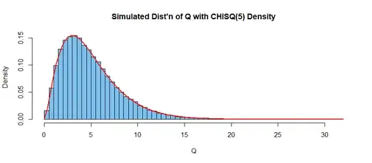
Many experiments. Now we seek to illustrate that $Q$ has very nearly the claimed chi-squared distribution, which has $E(Q) = 5$ and $Var(Q) = 10.$ We do many 600-roll experiments in order to get an idea of the distribution of $Q.$

set.seed(4321)
m = 10^5;  Q = numeric(m);  n = 600;  E = 100
for(i in 1:m) {
  X = rle(sort(sample(1:6,n,rep=T)))$lengths
  Q[i] = sum((X-E)^2/E) }
mean(Q);  var(Q);  quantile(Q, .95)
## 5.004733  # aprx E(Q) = 5
## 9.973967  # aprx Var(Q) = 10
##    95% 
##  11.02    # aprx c with P(Q < c)=.95;  c = 11.07
hist(q, prob=T, br=50, col="skyblue2", main="Simulated Dist'n of Q with CHISQ(5) Density")
curve(dchisq(x, 5), add=T, lwd=2, col="red")

The histogram below shows 100,000 values of $Q$ and the red curve is the density of $\mathsf{Chisq}(df = 5).$

The theory that supports the approximate chi-squared distribution of $Q$ is asymptotic. Simulation studies have shown that the approximation is useful for doing goodness-of-fit tests, provided there are enough 'rolls of the die' so that $E > 5,$ which is certainly true here.