Here are miscellaneous comments, perhaps you will find that some of them
help your intuition.
Moment generating functions multiply. Suppose $X, Y \sim \mathsf{Exp}(1),$ independently. Then each random
variable has MGF $m(t) = (1 - t)^{-1}.$ and the MGF of $T=X+Y$ is
$$m_T(t) = m_X(t)m_Y(t) = (1 - t)^{-2},$$ which is the MGF of $T \sim Gamma(2,1).$
Means match. $E(X) = 1, E(Y) = 1, E(X + Y) = E(T) = 2.$
Suppose you are first in line waiting for service. The server takes an
exponential length of time $X$ with $E(X) = 1$ to serve a customer (or
the s/he serves customers at an average rate of 1 per minute).
Because of the no-memory property of the exponential distribution,
the time before you begin being served is $X.$ Then the length
of time for you to be served is $Y,$ and the total time before you
can be on your way is $T = X+ Y$ with $E(T) = 2.$
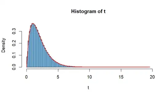
Simulation suggests distribution. Simulate a million sums $T,$ plot
the histogram of these totals, and note that the pdf
$f_T(x) = xe^{-x}$ for $x > 1,$ of $\mathsf{Gamma}(2,1)$
matches the histogram very well. (The code below is for R statistical
software.)
x = rexp(10^6, 1);  y = rexp(10^6, 1);  t = x + y
hist(t, prob=T, br=100, col="skyblue2")
curve(x*exp(-x), 0, max(t), add=T, lwd=2, col="red")
Consider joint density. The joint density function of $X$ and $Y$ is $f_{X,Y}(x,y) = e^{-(x+y)},$ for $x, y > 0.$ Based on 100,000 of the pairs simulated above, the
density of points plotted suggests the shape of the joint density function.
The area beneath the diagonal green line includes the points for $P(T \le 3) \approx 0.8,$
which can be evaluated by an integral. More generally, you can integrate to find
the CDF $F_T(x) = P(T \le x)$ and differentiate that to find the PDF $f_T.$
plot(x, y, pch=".", xlim=c(0,12), ylim=c(0,12), main="Scatterplot of (X, Y)")
abline(a=3, b=-1, col="green", lwd=2)

Notes: (1) Exponential and gamma distributions can be parameterized using either
the mean/scale $\beta$ or the rate $\lambda = 1/\beta.$ (R uses the rate.) For simplicity here, I have chosen to use
$\beta = \lambda = 1.$
(2) The sum of two exponential random variables is gamma only if the exponential random variables have the same rate (mean). Otherwise, the situation is
somewhat messier mathematically and also less intuitive.
(3) This paper treats the case
where $n$ exponentials are summed. You can set $n = 2$ when reading it.
The case with different parameters is considered first, then the case with
equal parameters.

