Answering, some time ago, to this question : Change in eigenvalues on changing one entry of a matrix, I had the idea of a graphical representation of roots of polynomial equations $$P(x,a)=P_{a}(x) \in \mathbb{R}[a,x]=\mathbb{R}[a][x],$$ such as
$$x^3+a x^2+(2a+1)x-3a=0.$$
[In fact, I will use notation $\lambda:=x$, because we can assume WLOG that such polynomials can always be considered as characteristic polynomials of certain matrices whose coefficients are polynomials in $a$ (companion matrix for example).]
The idea I have had is to build a simultaneous graphical representation of real and complex roots $\lambda_1,\lambda_2 ... \lambda_n$ of $P_a(\lambda)=0$ displaying their global dependency on real parameter $a$ (see Fig. 2).
This representation will be explained through an example [with a certain similarity with the example given in the reference] in order to convey easily the underlying ideas.
Let us consider the characteristic polynomial of the following matrix with one of its entries considered as a variable, here the bottom left entry (it is a particular case of what is called a pencil of matrices) :
$$A=\left(\begin{array}{rrrr}1& 3& 0& -2\\ -1& -2& 0& 3\\ -1& 2& -2& -2\\ \color{red}{a} & 3 & 0 & 0 \end{array}\right).\tag{1}$$
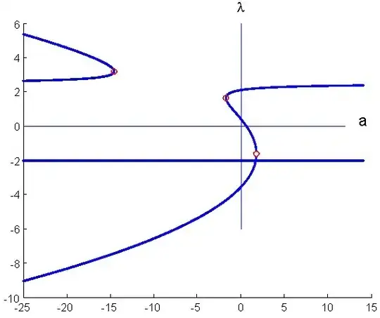
The real roots of characteristic polynomial $\det(A-\lambda I)=0$ are graphically represented on Fig. 1 : for a given value of $a$, the plotted points are $(a, \lambda_k)$. We see regions with two or four real roots, exceptionnaly 3. The eye is attracted by the generated "interweaved" curves that will be analyzed later on.
Fig. 1 : The "3 roots" case corresponds to places of bifurcation (little red circles) where 2 formerly distinct real roots coalesce, then "disappear" ; or, in a reverse way, appear "from scratch".
Let us proceed by showing how these appearances/disappearances (coalescence of real roots into a pair of complex conjugate roots) can be made visible.
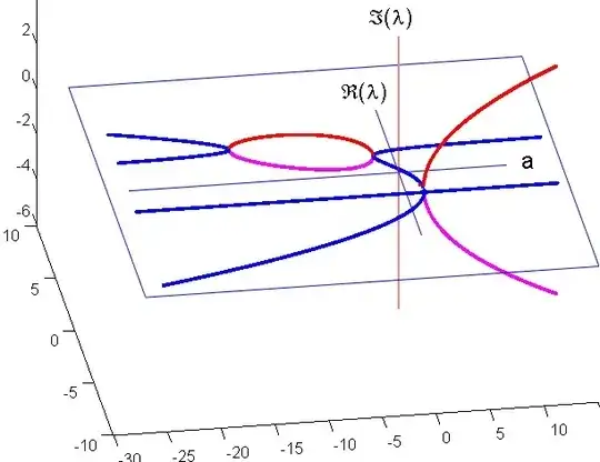
Take a look at (3D) Fig. 2, and compare it with (2D) Fig. 1. Instead of having a real-valued axis for $\lambda$, we switch to a "complex valued axis", more precisely, we replace a single axis by two of them, one for the real part, the other one for the imaginary part. As complex eigenvalues come by conjugate pairs (the polynomials we consider have real coefficients), Fig. 2 is symmetrical with respect to the horizontal plane defined by $a$ and $\Re(\lambda)$ axes.
In this way, we can "track" the roots and understand in a finer way what happens for certain values of the parameter.
Our understanding of Fig. 1 can be refined : see Appendix below.
Fig. 2. "Complexification" of Fig. 1. In order to gain a better 3D perception, here is a chinese poetic interpretation : imagine the blue lines as borders of a lake connected by a red bridge with a leaning weeping willow trunk and their magenta reflections on the lake...
Here is a second example (Fig. 3), associated with matrix :
$$A=\left(\begin{array}{rrrr}0& 1& 0& \color{red}{-a}\\ 1& 0& 1& 0\\ 0& 1& 0& 1\\ \color{red}{a} & 0 & 1 & 0 \end{array}\right).$$
Fig. 3.
I have willingly taken simple examples with at most first degree entries in parameter $a$ in order to demonstrate the interest of this approach. I have tried different cases, some of them with higher degrees. Representations analogous to Fig. 2 and Fig. 3 display, rather often, features with heuristical/pedagogical interest.
Question : This representation is very likely to be found elsewhere and/or linked to a certain already developed theory (differential geometry, Galois theory...). Can somebody give me an answer or at least a track ?
Remark : this representation is in fact very natural if one considers "level slices" at $a$= constant has the representation of the roots' position in the complex plane (see the comment of @Andrea Marino).
Edit: another pretty example is displayed on Fig.4.
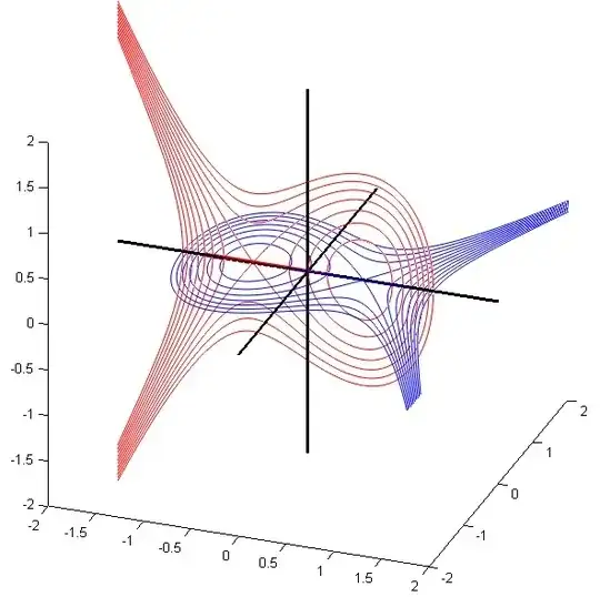
Fig. 4. Interweaving of a family of cubic curves with its own copy, one in a horizontal plane, the other one in a vertical plane.
It deals with the complex cubic equation under one of its standard forms (see the article by Milnor here):
$$z_2^2-z_1^3+z_1=t\tag{*}$$
where $$z_1=x_1+iy_1, z_2=x_2+iy_2 \in \mathbb{C}, t \in \mathbb{R}.$$
Let us consider the "slice" of this locus defined by $y_1=0$
Relationship (*) is equivalent in this case to the 2 equations
$$\begin{cases}-x_1^3+x_1+x_2^2-y_2^2-t&=&0\\x_2y_2&=&0\end{cases}$$
Considering the two cases $x_2=0$ or $y_2=0$, we get two cubic curves equations:
$$\begin{cases}\text{if} \ y_2=0 : & -x_1^3+x_1-t=-x_2^2\\\text{if} \ x_2=0: & -x_1^3+x_1-t=y_2^2\end{cases}$$
represented in Fig. 4 wrt axes $x_1,x_2,y_2$ for different values of $t$.
We find here once again this connexion between horizontal and vertical branches. The bifurcation occurs when $ -x_1^3+x_1-t$ has a sign change. Besides, limit cases corresponding to double points occur when $t=\pm \frac{2 \sqrt{3}}{9}$.
Edit : Meanwhile, I have found some references:
"Coupling of eigenvalues of complex matrices at diabolic or exceptional points" A.A. Mailybiev, O.N. Kirillov, A.P. Seyranian,
https://arxiv.org/pdf/math-ph/0411024.pdf (to be found as well here). See as well here."Complex Bifurcation from Real Paths" by M. E. Henderson and H. B. Keller, SIAM J. Appl. Mat. Vol. 50, No. 2, pp. 460-482, April 1990, that can be uploaded here.
And this special approach..
This one: Visualising Complex Polynomials A Parabola Is but a Drop in the Ocean of Quadratics, by H. Wiggins, A. Harding, J. Engelbrecht.
I mention also "Eigenvalue attraction" by R. Movassagh (https://arxiv.org/pdf/1404.4113.pdf), with a different point of view.
Appendix : A deeper understanding of Fig. 1:
The two "complex domain curves" (red, and magenta for their complex conjugate parts) are
on the right, a parabolic arc, thus planar, whereas,
on the left, the ellipse-looking curve is not planar.
Consider now the (blue) real components (the straight line, and the two curves of the horizontal plane); let us play a game of anticipation:
for the straight line, we guess the presence of a root $\lambda=-2.$
for the two curves, it is natural to consider them together as having the same equation with a common horizontal asymptote for a certain value (of course never reached) of $\lambda$. Zooming, one can guess that this asymptote is characterized by $\lambda_{\infty}=2.5$, Besides, a little observation makes evident a parabolic envelope ; gathering these observations, a possible equation for $a$ as a function of $\lambda$ is as follows :
$$\tag{1}a = p\lambda^2+ q\lambda +r+\dfrac{s}{\lambda-2.5}.$$
for certain coefficients $p,q,r,s$. It remains to check (1) by examining the factorization of the characteristic polynomial of $A$ and then its roots. Using a CAS, or by hand calculation, we obtain:
$$\tag{2}\det(A-\lambda I)=(\lambda+2)P(\lambda) \ \ \ \ \text{with} \ \ \ \ P(\lambda):=\lambda^3+\lambda^2-8\lambda+2a \lambda+3-5a$$
Equating (2) to zero, we obtain $\lambda=-2$, as awaited, or $P(\lambda)=0$, which can be written in the following equivalent way :
$$a=\dfrac{-\lambda^3-\lambda^2+8\lambda-3}{2 \lambda -5}$$
in full conformity with form (1).


