The pdf (or pmf) of $\mathsf{Pois}(\lambda)$ is $f(x|\lambda) = e^{-\lambda}\lambda^x/x!,$ for $\lambda > 0$ and $x = 0, 1,2, \dots .$
The likelihood of a sample $\mathbf{x} = (x_1, x_2, \dots, x_n)$ is defined as the product
$$f(\mathbf{x}|\lambda) = \prod_{i=1}^n f(x|\lambda) =
\prod_{i=1}^n \frac{e^{-\lambda}\lambda^{x_i}}{x_i!} =
\frac{e^{-n\lambda}\lambda^{\sum_i x_i}}{\prod_i x_i!}
= \frac{e^{-n\lambda}\lambda^t}{\prod_i x_i!} \propto e^{-n\lambda}\lambda^t,$$
where $ t = \sum_{i=1}^n x_i$ is the total of the $n$ observations.
Also, in this setting $f(\mathbf{x}|\lambda)$ is viewed as a function
of the variable $\lambda$ for fixed observed values of the $x_i$ and $t.$
It is customary to specify a likelihood function 'up to a constant factor',
so in the last step of the displayed equation we have dropped the constant
in the denominator. [The symbol $\propto$ is read "proportional to".]
The log-likelihood is the logarithm (usually the natural logarithm) of the likelihood function, here it is
$$\ell(\lambda) = \ln f(\mathbf{x}|\lambda) = -n\lambda +t\ln\lambda.$$
One use of likelihood functions is to find maximum likelihood
estimators. Here we find the value of $\lambda$ (expressed in terms of the data)
that maximizes the likelihood function $f(\mathbf{x}|\lambda).$
Maximizing $\ell(\lambda)$ accomplishes the same goal. For Poisson data
we maximize the likelihood by setting the derivative (with respect to $\lambda)$
of $\ell(\theta)$ equal to $0$, solving for $\lambda$ and verifying that
the result is an absolute maximum.
The derivative of the log-likelihood is $\ell^\prime(\lambda) = -n + t/\lambda.$
Setting $\ell^\prime(\lambda) = 0$ we obtain the equation $n = t/\lambda.$
Solving this equation for $\lambda$ we get the maximum likelihood
estimator $\hat \lambda = t/n = \frac{1}{n}\sum_i x_i = \bar x.$ I will leave
it to you to verify that $\bar x$ is truly the maximum.
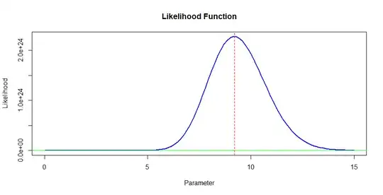
Example: Suppose we get the $n = 5$ values $12, 5, 12, 9, 8,$ which
sum to 46 and which have a sample mean $\bar x = 9.2.$ Then the likelihood function is
$f(\mathbf{x}|\lambda) = e^{-5\lambda}\lambda^{46}.$ The graph below illustrates the maximum of the likelihood curve does indeed occur at $\hat \lambda = 9.2.$
[The five observations were simulated from $\mathsf{Pois}(\lambda=10),$ so
$\hat \lambda = 9.2$ is not a bad estimate of $\lambda$ using only $n = 5$
observations.]