23

I'm working on an engineering project, and I'd like to be able to input an equation into my CAD software, rather than drawing a spline.

The spline is pretty simple - a gentle curve which begins and ends horizontal.

Is there a simple equation for this curve?
Or perhaps two equations, one for each half?
I can also work with parametric equations, if necessary.

spline curve

Giffyguy
  • 679

11 Answers11

35

These splines are usually drawn as Bézier curves. Specifically, since it is defined by four points, the curve is a cubic Bézier. $$\vec{x} = (1-t)^3\vec{P_0} + 3(1-t)^2t\vec{P_1} + 3(1-t)t^2\vec{P_2} + t^3\vec{P_3}$$ with \begin{align} \vec{P_0} &= (-60, 20),\\ \vec{P_1} &= (0, 20),\\ \vec{P_2} &= (0, -20),\\ \textrm{and}\ \vec{P_3} &= (60, -20). \end{align} The variable $t$ is $0$ at the left end of the curve and $1$ at the right end. With these points, the origin is in the center of the figure. Taking $x$- and $y$-coordinates separately, we have \begin{align} x(t) &= -60(1-t)^3 + 60t^3\\ y(t) &= 20(1-t)^3 + 60(1-t)^2t - 60(1-t)t^2 - 20t^3. \end{align} After some arithmetic, these simplify to \begin{align} x(t) &= 60(2t^3 - 3t^2 + 3t - 1)\\ y(t) &= 20(4t^3 - 6t^2 + 1). \end{align}

I've overlapped the curves below to show that they match. The green is the original curve from your picture; the blue is the curve from the equations above. Overlapping curves

Mark H
  • 1,322
  • @Giffyguy: Or, if you rather replicate my curve for $(0,40)$ to $(120,0)$, use control points $(0,40), (40,40), (80,0), (120,40)$; or, $(-60,20), (-20,20),(20,-20), (60,-20)$ if center is at origin. That would be the Bézier variant with $x$ linear, you see. Moving the center control points along the $x$ axis, antisymmetrically, will modify the steepness of the curve in the center. – Nominal Animal Apr 20 '16 at 04:37
  • 1
    My guess would have been that the nodes we see in the picture are the control points ... So $(-60,20), (0,20), (0,-20), (60,-20)$? – Hagen von Eitzen Apr 20 '16 at 08:21
  • https://pomax.github.io/bezierinfo/ – BlackBear Apr 20 '16 at 09:57
20

You could try a sine or cosine wave. Taking the lower left corner as the origin, let $$y=20\cos\left(\frac {\pi x}{120}\right)+20$$

This can also be written as $$y=40\cos^2\left(\frac{\pi x}{240}\right)$$

David Quinn
  • 35,087
  • A neat solution too. Not very far from the cubic equation as represented here. – Raymond Manzoni Apr 19 '16 at 22:27
  • This isn't the exact answer to my question (the way it's worded), but it's the solution I ended up using, since it produces a maximally smooth curve - smoother than the cubic Bézier was. Thanks for the help! – Giffyguy Apr 20 '16 at 22:39
  • You're welcome. Pleased to be of help. – David Quinn Apr 20 '16 at 22:45
  • @Giffyguy You might want to consider that using a trigonometric function often is way slower than some basic arithmetic operations. So if you have to call this often, using Mark H's answer can improve speed. – Alfe Apr 21 '16 at 09:57
  • 1
    @Giffyguy I'm curious about what you mean by "maximally smooth." What's your definition/criteria? – Mark H Apr 21 '16 at 10:36
  • @Alfe Good point, worth noting for software developers. I am a software developer, but right now I'm working on a mechanical engineering project using CAD software. In this context, mechanical functionality and accuracy are more important than computing speed. – Giffyguy Apr 21 '16 at 17:11
  • @MarkH (1 of 3) I didn't want to go into too much detail, because it gets really confusing really fast. Short version: air is flowing over this shape in the horizontal direction, and aerodynamic efficiency is important. In this context, it's important to remove sharp angles, which is why I don't just make it a straight diagonal line connecting two horizontal lines. – Giffyguy Apr 21 '16 at 17:54
  • @MarkH (2 of 3) So the gentlest possible curve is what I was looking for, and I was using splines because I didn't understand the math involved and figured splines (cubic) would be OK. Turns out, when compared directly, the trig version is more "gradual." As far as I can tell, the trig version appears to be as gradual as it is possible to be, hence "maximally." – Giffyguy Apr 21 '16 at 17:54
  • @MarkH (3 of 3) The way I figure this is, if you create two vertical ellipses, bind them to both the origin and the horizontal peaks of my curve, then stretch their height to infinity, the result would appear to be the cosine wave. Helpful diagram here. I don't know the calculus, but am I on the right track here? – Giffyguy Apr 21 '16 at 17:54
  • @Giffyguy An infinitely stretched ellipse is a parabola. See Jaume Oliver Lafont's answer and my second answer for the result of your joined ellipses. – Mark H Apr 22 '16 at 12:11
14

Most of the other responses will, outside the given range, be either: (a) cyclical (come back up & down repeatedly), or (b) diverge to +/- infinity at the limit (far away from the origin). If it's at all important that the tails have horizontal asymptotes in the limit, then you want some flavor of logistic function:

$$f(x)= \frac{L}{1+e^{-k(x-x_0)}}$$

Graph of logistic function

  • 4
    Note, though, that this function doesn't go to a "nice" value at any particular value of $x$; for example, if I want $f(-4) = 0$ and $f(4) = 1$, you'll have to offset the function by an additive constant, and the values of $L$ will be some complicated expression in terms of exponentials. This is really the flip-side of the problem you point out: this function automatically has nice behavior outside the interval, but is uglier if you want precise control at the boundaries of the interval. – Michael Seifert Apr 20 '16 at 17:01
  • 4
    This is also referred to (often in computer science) as a sigmoid curve https://en.wikipedia.org/wiki/Sigmoid_function – mike Apr 21 '16 at 13:43
11

Assuming you mean $$\begin{align} y(0) &= 40 \\ y(120) &= 0 \\ \dot{y}(0) &= 0 \\ \dot{y}(120) &= 0 \end{align}$$ then a simple cubic will do: $$y(x) = \frac{x^3}{21600} - \frac{x^2}{120} + 40$$

At range $x=0\dots120$, it looks like this: Cubic example curve


You can find these very easily. In general, a cubic curve is $$y(x) = C_3 x^3 + C_2 x^2 + C_1 x + C_0$$ and its derivative $$\dot{y} = \frac{d y(x)}{d x} = 3 C_3 x^2 + 2 C_2 x + C_1$$ Fix four values, each fixing one of the constants, and that's it.

  • I obtained $\boxed{ \displaystyle P(x) = \frac{x^3}{21600} - \frac{x}{2}}$ with the same method (with the derivative proportional to $x^2-60^2$). – Raymond Manzoni Apr 19 '16 at 21:51
  • @RaymondManzoni I think that is even negative in parts the function in the question is positive...If at all, I thinkl it should be $;-x^3;$ and some coefficients here and there. – DonAntonio Apr 19 '16 at 21:53
  • my solution is centered at $0$ it may of course be shifted up by adding $20$ and/or translated by replacing $x$ with $x-x_0$... – Raymond Manzoni Apr 19 '16 at 21:54
  • @Joanpemo It's fine if they go negative, I can easily transform to place the origin wherever I need it. Apart from that, I'm still tinkering with the information to see how it operates. Do you see any major problems? – Giffyguy Apr 19 '16 at 21:55
  • @Giffyguy: would you wish to go to infinity instead of stopping at $\pm 60$ then you could try one of the sigmoid functions. (btw the solution here (+1) is the same as mine with $x\to x-60$ and $20$ added). – Raymond Manzoni Apr 19 '16 at 22:01
  • @Giffyguy: The slope of the above curve is $0$ at both ends. So, even if you continue them with straight lines, you'll have $C^1$ continuity. – Nominal Animal Apr 19 '16 at 22:14
  • For searching purposes: what was constructed here is a cubic Hermite interpolating polynomial. Usually does a nice job if the derivative values are sanely chosen. – J. M. ain't a mathematician Apr 20 '16 at 00:31
  • 1
    @Joanpemo What do you mean by "twisted brother"? It seems like a normal cubic to me: what's wrong with it? –  Apr 20 '16 at 03:39
  • @J.M. Exactly, although here, the interpolating polynomial is the important part. It also happens that a cubic Bézier curve of form $$x(t) = X_0 (1-t)^3 + X_1 3 (1-t)^2 t + X_2 3 (1-t) t^2 + X_3 t^3$$is linear if and only if $X_1 = (X_0 + 3 X_3)/4$ and $X_2 = (3 X_0 + X_3)/4$, and that all cubic Béziers can be written as normal cubic polynomials as $$x(t) = (X_3 - 3X_2 + 3X_1 - X_0) t^3 + (3 X_2 - 6 X_1 + 3 X_0) t^2 + (3 X_1 - 3 X_0) t + X_0$$. – Nominal Animal Apr 20 '16 at 04:45
  • The above is interesting if you wish to work with polynomials and cubic Béziers. CAD programs often work well with polynomials (and typically internally use cubic Bézier curves a lot, as well as cubic Bézier patches to describe surfaces in 3D), because they behave nicely and are easy to compute. – Nominal Animal Apr 20 '16 at 04:48
  • Certainly, the basis changes between the Hermite and Bézier systems are well-known to those who know them. :) In any case, sigmoids such as the OP's are very cheaply constructed as appropriate interpolating polynomials with prescribed derivatives, and your procedure is the most straightforward way to go about it. As another aside: computer graphics buffs may be more familiar with this as (an appropriate rescaling of) the smoothstep() function. – J. M. ain't a mathematician Apr 20 '16 at 05:20
  • @J.M. I find myself using $3 t^2 - 2 t^3$ as interpolation between $0$ and $1$ every now and then; its curvature is nice. For movement, $6 t^5 - 15 t^4 + 10 t^3$ is even nicer, as it has $C^2$ continuity (first and second derivatives zero at $t=0$ and $t=1$); it has not only smooth "velocity", but smooth "acceleration", like best new elevators. The equivalent $C^2$ smooth curve the OP is asking, for $x=0,y=40$ to $x=120,y=0$, would be $$y(x) = -x^5 / 103680000 + x^4 / 345600 - x^3 / 4320 + 40$$. – Nominal Animal Apr 20 '16 at 05:41
9

I assume origin is at middle of vertical y-axis line. Mathematica code and plot:

Plot [ 20 Cos[ Pi x/120], {x, 0, 120}, AspectRatio -> 1/3, GridLines
-> Automatic, PlotStyle -> Thick]

$$ y = 20 \cos \frac{\pi x}{120} ,\, (0<x<120). $$ CosCurveMathematica

EDIT1:

Or a cubic whose domain/range box dimension can be varied:

$$ \dfrac{y}{x}= \dfrac{3b}{2a}\big(\dfrac{x^2}{3 a^2}-1\big) $$

enter image description here

  a = 60; b = 20;
  Plot[3 b/(2 a ) \,x \;( x^2/(3 a^2) - 1) , {x, -a, a}, PlotStyle -> {Thick, Blue}, AspectRatio -> 0.2, GridLines -> Automatic, AxesLabel -> {X, Y}, GridLinesStyle -> Directive[Gray]]
Narasimham
  • 42,260
  • This isn't the exact answer to my question (the way it's worded), but it's the solution I ended up using, since it produces a maximally smooth curve - smoother than the cubic Bézier was. Thanks for the help! – Giffyguy Apr 20 '16 at 22:40
  • Ok but wonder what exactly is needed for an acceptable answer. We can for example set it so that the central max slope is manipulable as a variable using boundary values in odes, right from saw tooth to diagonal line. – Narasimham Apr 20 '16 at 22:54
  • 1
    This answer is fabulous, and I'm using it as my final solution. It just so happens that the explicit wording of my question technically asks for the cubic Bézier (even though I didn't realize that was its name at the time). That's the reason I accepted Mark H's answer. – Giffyguy Apr 20 '16 at 22:58
5

Using elementary functions, one that roughly approximates your diagram is $f(x)=-\frac{40}{\pi}\arctan(\frac{x}{10})+20$. It isn't a great fit, but a rough approximate.

Using non-elementary functions, your plot looks really similar to a mirrored normal distribution cumulative curve, which is based on the error function and defined as $\mathbb{erf}(x)=\frac{2}{\sqrt{\pi}}\int_0^x e^{-t^2}dt$. Your diagram could be modeled with this, and it looks like it would fit more closely than the elementary function attempt: $f(x)=-20\mathbb{erf}(\frac{x}{30})+20$.

These models are based off of $f(0)=20$, although they easily could be shifted to fit whatever value you would like for $f(0)$.

Ethan Hunt
  • 1,053
3

It does look a bit like $-\tan^{-1}x$ if you were searching a similar looking curve. I think that modifying the equation a bit : like multiplying it by some constant k and taking the curve from $[-x,x]$ and x does not tend to $\infty$ would result into the part of the curve you have shown

I think you can figure out the rest for yourself. Good Luck!

brainst
  • 269
3

With two equations, a parabola can be used for each half.

Imposing the three conditions $$f(0)=0,$$ $$f(60)=-f(-60)=-20,$$ and $$f'(60)=f'(-60)=0$$

results in the expression $$f(x)=\frac{x^2 sgn(x)}{180}-\frac{2x}{3},$$

where $sgn(x)$ is the sign function.

The slope is $-\frac{2}{3}$ at the origin (see the graphic here).

  • 1
    What is the value of sgn(0)? – Stephan Apr 21 '16 at 11:40
  • From the condition of odd function sgn(x)=-sgn(-x), then it has to be 0. But in this case, since it is multiplying the zero from x^2, choosing -1,0 or 1 would not make any difference, would it? These three references use sgn(0)=0. http://mathworld.wolfram.com/Sign.html https://en.wikipedia.org/wiki/Sign_function http://oeis.org/A057427 – Jaume Oliver Lafont Apr 21 '16 at 18:44
3

I am an professional electrical engineer (according to the gubbermint of California), so I will give you an engineer's answer that is sure to be offensive to the math people here.

Download a program called "Curve Expert" Just get the basic program, not the professional version. Input your data, and you will get a better fit than you want. From your graph, it could be a sinusoid, a polynomial, an inverse hyperbolic sine, a rational function, something built from the cumulative normal distribution, or some kind of logistic function.

Curve expert will help you decide what is best. You will probably fall in love with it and buy the license when the trial period expires.

*** disclaimer: I have used curve expert for years, but have no financial, romantic, political, or other interest in it.

richard1941
  • 1,051
2

There are many alternatives, and you didn't give us enough information to choose between them intelligently. So, here are a few options; you can choose.

I assume that the coordinate system origin is at the center of the curve.

(1) Parametric Cubic in Bézier Form
This is the obvious choice because the symbols on your picture look like the control points of a cubic Bézier curve. These control points are $\mathbf{P}_0 = (-60,20)$, $\mathbf{P}_1 = (0,20)$, $\mathbf{P}_2 = (0,-20)$, and $\mathbf{P}_3 = (60,-20)$. Then the curve is $$ \mathbf{P}(t) = (1-t)^3 \mathbf{P}_0 + 3t(1-t)^2 \mathbf{P}_1 + 3t^2(1-t) \mathbf{P}_2 + t^3 \mathbf{P}_3 $$ In fact, more generally, you can take $\mathbf{P}_1 = (-k,20)$, $\mathbf{P}_2 = (k,-20)$, and you'll still get a curve of roughly the desired shape. You can adjust $k$ to get exactly the shape you want.

(2) Real-Valued Cubic in Algebraic Form
If you're going to use the curve as a "law" to control variation of some variable, then you want it to be in the form of a real-valued function $y=f(x)$. The parametric equation given above is inconvenient because, given a value of $x$, it's not easy to find the corresponding value of $y$. A suitable equation is: $$ y = px(x^2 - q) $$ Using the relations $y(60) = -20$ and $y'(60)=0$, you can calculate $p$ and $q$.

(3) Real-Valued Cubic in Bézier Form
Another option is to write the equation in Bézier form, again. If we let $u = \tfrac{1}{120}(x+60)$, then $u= 0$ when $x=-60$ and $u=1$ when $x=60$. The equation of the curve is $$ y = a(1-u)^3 + 3au(1-u)^2 - 3au^2(1-u) - au^3 $$ where $a=20$. In a CAD system, you can construct this curve by using the control points $\mathbf{P}_0 = (-60,20)$, $\mathbf{P}_1 = (-20,20)$, $\mathbf{P}_2 = (20,-20)$, and $\mathbf{P}_3 = (60,-20)$. So, this is the case $k=20$ of #1 above.

(4) Real-Valued Quintic in Bézier Form
One problem with the real-valued cubics is that they give you no freedom to adjust the shape of the curve. To get some adjustment freedom, you can use a quintic curve, instead. Again, it's easiest to write this in Bézier form. So, as before, we let $u = \tfrac{1}{120}(x+60)$. Then the equation of a suitable quintic is $$ y = a(1-u)^5 + 5au(1-u)^4 + 10bu^2(1-u)^3 - 10bu^3(1-u)^2 - 5au^4(1-u) - au^5 $$ 
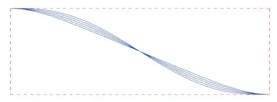
where $a=20$, again. You can change the value of $b$ to adjust the shape of the curve. In your CAD system, you can construct this curve using the control points $\mathbf{P}_0 = (-60,20)$, $\mathbf{P}_1 = (-36,20)$, $\mathbf{P}_2 = (-12,b)$, $\mathbf{P}_3 = (12,-b)$, $\mathbf{P}_4 = (36,-20)$, and $\mathbf{P}_5 = (60,-20)$. The particular choice $b=20$ gives you a curve whose second derivatives are zero at the start and end, which may have some merit in your application. Here are curves with $b = 0,5,10,15,20$.

enter image description here

(5) Quadratic B-spline
Using four control points (like the ones described in #1 or #3), you can define a b-spline curve of degree 2 (i.e. quadratic) that has two segments. Each quadratic segment will actually be a parabola, so the solution is then two parabolas joined end-to-end with tangent continuity. There will be a discontinuity of curvature at the inflexion point where the two pieces meet, and this might be a problem in an aerodynamics application. None of the other solutions I listed have this problem.

(6) Trigonometric Solutions
Several people gave solutions using trigonometric functions. I don't recommend these. CAD systems usually support only polynomial and rational curves (Bézier curves and NURBS curves). They don't support curves described by trigonometric functions. So, if you use trig functions, you will have to approximate, and you'll end up with a spline curve with many segments and wiggly curvature, which will be bad for aerodynamics. All the curves I suggested above can be exactly represented in a typical CAD system, so they don't have this problem.

bubba
  • 44,617
  • Thanks for detailing each of these. I just have to say for #5, I've only ever used one particular CAD system, AutoDesk Inventor, which does support trig curves with none of the problems you mentioned. However, this may not be the case for other CAD systems, so that info might be good for other people reading over this. However, I'm currently comparing parabolas to the trig solutions, and I'll probably switch to parabolas anyway, since they are more certainly what I am looking for - with the bonus of being polynomial/rational functions, as opposed to the trig solutions. – Giffyguy Apr 22 '16 at 15:20
  • I'm surprised Inventor supports trig curves. They're not supported by data exchange standards like IGES or STEP. Are you sure they don't get approximated by splines? Two parabolas joined end-to-end would work. In fact, this would be a b-spline of degree 2 with 2 segments. You can define this curve using the same control points as in #1. – bubba Apr 23 '16 at 00:20
1

Note: Now that I've finished this derivation, I see it's the same as Jaume Oliver Lafont's answer. Perhaps some extra justifications will be useful.

In looking over @Giffyguy's comments on other answers, it seems the real goal is to have a curve with minimum curvature or maximum smoothness. I'll take this to mean the maximum absolute value of the second derivative should be minimized. The way to minimize the second derivative everywhere is to make it everywhere constant, which means we're dealing with a parabola $$y(x) = ax^2 + bx + c$$ with constraints $$y(0) = 0$$ $$y(60) = -20$$ for the right half, and $$y'(60) = 0.$$

The first constraint means $c = 0$. The second and third constraints result in, respectively, $$a(60)^2 + b(60) = -20.$$ $$2a(60) + b = 0$$ Solving results in $a = \frac{1}{180}$ and $b = \frac{2}{3}$. So, $$y = \frac{1}{180}x^2 - \frac{2}{3}x = \frac{x(x-120)}{180}$$

The second derivative has a constant value of $1/90$, which is smaller than the maximum value of the second derivative of the cosine functions ($1/60$) and the cubic polynomial ($\approx 1/72$). The function spanning the full width would be $$y(x) = \left\{ \begin{array}[ll] \\ -\frac{x(x+120)}{180} & x \lt 0 \\ \frac{x(x-120)}{180} & x \geq 0 \\ \end{array} \right.$$

Mark H
  • 1,322
  • Thanks for going the extra mile. This is kind of an XY problem, it seems, and my question was very brief. I'll leave your Bézier answer as the accepted answer, since the question is worded the way it is. – Giffyguy Apr 22 '16 at 16:31
  • After several hours dealing with support forums for my CAD software, it was determined that my CAD software does not support the Sign function (or the Abs function, oddly enough). So I'm doubly grateful that you also split the equations out into two halves, one for each sign. It's a little obnoxious that I have to plot two curves, simply because it will interfere with the flexibility of the drawing down the road, but I've got nobody to blame except the CAD developers. :) – Giffyguy Apr 22 '16 at 18:59
  • @Giffyguy If the problem with the sign function from this list is that it is defined as 0 for negative and 1 for positive, the standard sign between -1 and 1 is $2sign(x)-1$. – Jaume Oliver Lafont Apr 24 '16 at 23:19