8

Background:

SmoothStep is a simple sigmoid-like function defined as S(x) = 3x^2 - 2x^3. It is monotonically increasing from (0, 0) to (1, 1), is rotationally symmetric over that interval, and has flat tangents at both endpoints. This function is useful for generating an interpolation parameter when you would like to ease in and out between an initial and final value.

S(S(x)) will yield a function that has a longer ease-in/ease-out with a sharper transition in the middle, and S(S(S(x))) makes the middle steeper still. The more times the function is nested, the more protracted the ease is and the steeper the tangent at the midpoint becomes.

Question:

I would like to be able to drive this curve from shallow to steep continuously using some kind of 'steepness' parameter, but repeated iteration only allows discrete curves to be evaluated. Additionally, the cost of evaluating the function grows with the number of nested iterations. Is there any similar function which could be tuned continuously in this manner?
Jason
  • 440

6 Answers6

6

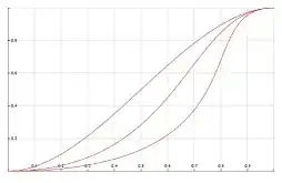
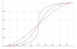
This graph exposes two parameters which allow the curve to be tuned continuously: https://www.desmos.com/calculator/3zhzwbfrxd.

enter image description here

Royi
  • 10,050
Jason
  • 440
  • Can this be modified to add a variable to set the Y position of the fulcrum? – troy_s Feb 13 '17 at 23:14
  • Given the symmetry of the construction I'm not sure there is an easy way to make that change. The blue and red graphs are uniformly scaled and rotated copies of each other, which forces the location where they meet to be on the y=x line. While you could scale each non-uniformly, doing so would break the tangent and create a discontinuity at the fulcrum. – Jason Hise Feb 14 '17 at 23:59
  • Actually maybe you can... there is already a parameter to control the slope, so you might be able to add an amount that the slopes are split and then undo that split with the scaling. I'll have to look again when I have a bit more time. – Jason Hise Feb 15 '17 at 00:55
  • 1
    @Jason, It would be great, for the completeness of the answer, if you wrote the function explicitly in the answer. The Desmos website might be unavailable one day. – Royi Sep 30 '23 at 12:59
  • This answer could be improved by including all relevant information in the answer itself, not just in external links or images. – Smiley1000 Dec 11 '24 at 08:40
2

How about $S(f_c(x))$ where $f_c(x)=(1-c)x+cS(x)$, $c\ge 0$?

  • I just tried plugging that into google, replacing c with y, as:

    z = 3((1-y)x + y(3x^2 - 2x^3))^2 - 2((1-y)x + y(3x^2 - 2x^3))^3

    It looks like you get nice curves from c = 0 to c = 1, but after that you get additional undesirable folds and begin to hit both 0 and 1 twice, rather than just at the endpoints.

    – Jason Apr 19 '16 at 07:01
  • 1
    Looking more closely at your answer, it looks like you are advocating a linear interpolation between S(S(x)) and S(x). I guess it is reasonable to lerp between adjacent curves, so you could use the floor of c to choose the number of nested iterations of S, and the fractional part to control the linear blend. I can implement it this way and it will probably work, but I was hoping to avoid iterating an unbounded number of times as c increases. – Jason Apr 19 '16 at 17:18
2

If you are willing to go with parametric representation for your curve, then this is pretty easy to achieve with the following:

$\begin{cases}x(t)=(t^3-2t^2+t)m_0+(-2t^3+3t^2)+(t^3-t^2)m_1 \\y(t)=-2t^3+3t^2 \end{cases}$

You can use $m_0$ and $m_1$ to separately control how strong the curve will go out of $(0,0)$ and into $(1,1)$. The following are two sample pictures: first one with $m_0=m_1=1,2,3$ and second one with $m_0=1,2,3$ and $m_1=1$.

enter image description here enter image description here

The permalinks for generating these pictures are below:

http://fooplot.com/plot/jtu07hy41r
http://fooplot.com/plot/muk7fu5ifi

fang
  • 3,630
  • That does look useful and I like that the ease in and out can be controlled independently. Unfortunately I do still need a mapping from a single variable, which in this case means solving for t in terms of x. It's a cubic, so it should be possible to subtract x from both sides and then find the roots... I'll give it a shot later, no idea how messy it will get though. – Jason Apr 19 '16 at 20:58
  • As expected, when you ask wolfram alpha to solve for t in terms of x the closed form is a wall of text. This would require either using a dedicated cubic solver or searching the curve, and both of these options are likely to be too expensive to perform for each curve evaluation. – Jason Apr 21 '16 at 02:23
0

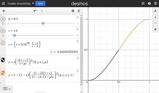
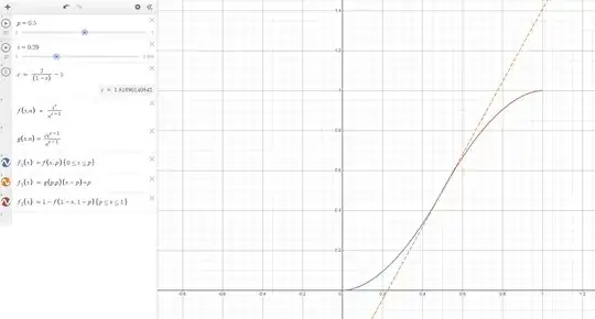
Jason's answer is nice, but I have an alternative formula that just uses $x^2$ instead of $x^n$, which might be desirable for programming implementation. It also fits closer to the original SmoothStep ($3x^2-2x^3$) function (using $p=0.5, s=1.5$).

$p$ = $x$ position of max slope

$s$ = slope at $p$

$$c = \frac{1-s}{s-3}$$ $$y = \begin{cases} x\left[\frac{x\left(1 + c\right)}{x + pc}\right]^2 &0 \le x \le p\\ 1 - \left(1-x\right)\left[\frac{\left(1-x\right)\left(1 + c\right)}{\left(1-x\right) + \left(1-p\right)c}\right]^2 &p \lt x \le 1 \end{cases}$$

https://www.desmos.com/calculator/gy3f8hvhvn

Desmos graph screenshot

0

If you're ok with using a non-polynomial, define

$$\begin{align} u(x) &= {{1}\over{1-x}} - {{1}\over{x}} \\ b(x) &= {{ 1 }\over{ 1 + e^{-kx/2} }} \\ S_{∞}(x) &= b(u(x)) \end{align}$$

That basically squishes a logistic function down into a $[0, 1]$ domain, so you have

$$\begin{align} 0 &= S_∞(0) \\ 0 &= S'_∞(0) = S''_∞(0) = S'''_∞(0) = ... \\ 1 &= S_∞(1) \\ 0 &= S'_∞(1) = S''_∞(1) = S'''_∞(1) = ... \\ \end{align}$$

But you also have

$$ S'_∞(½) = k $$

so you can choose how steeply transitions without changing the number of operations required to compute it.

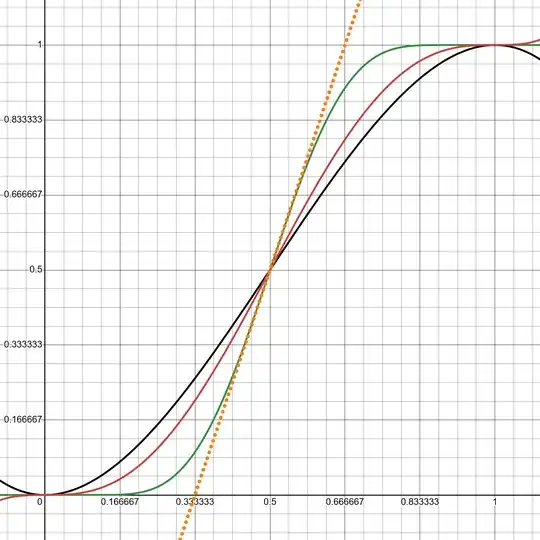
Demo with $k=3$: https://www.desmos.com/calculator/arzm40nawt Graph of S_1 S_2 and S_∞

me22
  • 201
0

If you're ok with a piecewise solution, this is easy to parameterize because it's exactly cubic Hermite interpolation.

Start by grabbing the basis functions:

$$\begin{align} B_{0}(x) &= 2x^{3}-3x^{2}+1 \\ B_{1}(x) &= x^{3}-2x^{2}+x \\ B_{2}(x) &= -2x^{3}+3x^{2} \\ B_{3}(x) &= x^{3}-x^{2} \\ \end{align}$$

(Aside: notice that $B_2$ is smoothstep, because it's just doing exactly this for the easy case of $f(0)=0, f'(0)=0, f(1)=1, f'(1)=0$ where those zeros remove all the other basis functions.)

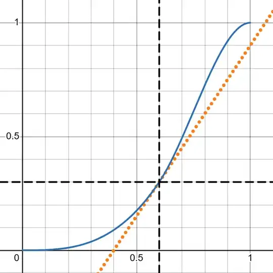
Then there's two cases if you want the curve to go through $(P,Q)$ with slope $M$:

The first, for $0≤x≤P$, has $f_1(0)=0, f'_1(0)=0, f_1(P)=Q, f'_1(P)=M$, so it's $$ f_1(x) = B_{2}\left(\frac{x}{P}\right)Q+B_{3}\left(\frac{x}{P}\right)MP $$

The second, for $P≤x≤1$, has $f_2(P)=Q, f'_2(P)=<, f_2(1)=1, f'_2(1)=0$, so it's

$$ f_2(x) = B_{0}\left(\frac{x-P}{1-P}\right)Q+B_{1}\left(\frac{x-P}{1-P}\right)M\left(1-P\right)+B_{2}\left(\frac{x-P}{1-P}\right) $$

Demo with sliders for $P$, $Q$, and $M$: https://www.desmos.com/calculator/nupvwjmawp graph for P=.6 Q=.3 M=1.5

Just beware that for some parameter choices it'll go outside the $[0, 1]$ range, particularly for aggressive slopes or if $(P, Q)$ gets too close to the edges. Also even if it stays in-range, it's still usually jerky: the acceleration is discontinuous, so this would be bad for something like a camera. (It's only non-jerky if it reduces to smoothstep, such as if $(P,Q)=(½,½)$ and $M=\frac{3}{2}$.)

me22
  • 201